ContourPlot has weird Jagged line

Question

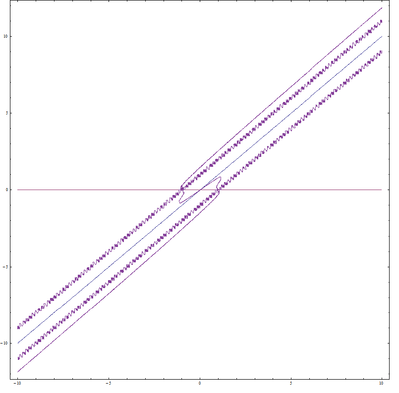
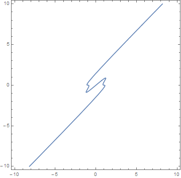
I'm trying to make a series of contour plots, but pretty much everything I try (and I've tried many different equations) ends up with at least one jagged line of the form seen in the image. I don't think these jagged lines are particularly meaningful (but I could be wrong), so it'd be nice if they were gone. I've tried using Exclusions, in a variety of formats (p>q, p<=q,True), but none of them seemed to work (they did get rid of some of the useful data which isn't helpful). Changing the number of PlotPoints doesn't particularly help, and it makes the code take forever to run. Here is the code that made the pasted image.

y = (p - q) + pg - m*h
ClearAll[m]

eq5 = p == q (1 + ρ 2 (1 + 3 y^2)/(1 - y^2)^3)
mset = 0;
ρset = .1;

table5 = Evaluate[
   Table[Evaluate@
     eq5, {pg, {0, 0}}, {m, {mset, 
      mset}}, {ρ, {ρset, ρset}}]];

plotpoints = 150;

fulltable = Flatten[Union[{table5, q == 0, p == q}]];

ContourPlot[Evaluate[fulltable], {p, -10, 10}, {q, -100, 100}, 
 PlotPoints -> plotpoints, PlotRange -> All, Exclusions -> True]

Answer 1

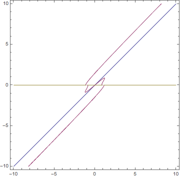
ContourPlot has trouble with discontinuous functions and the setting Exclusions -> True does not get the job done here. Let's help it out. When solving symbolic equations, it helps to have exact coefficients, so I'll use Rationalize on the equations in fulltable to compute the exclusions in excl.

plotpoints = 50;
fulltable = Union[Flatten[{table5, q == 0, p == q}]];

excl = Cases[
   FactorList /@ (Rationalize@fulltable /. 
      Equal -> Subtract), {poly_ /; ! NumericQ[poly], _?Negative} :> 
    poly == 0, Infinity];
(*
  {p == q, p == (1 + (0.2 (1 + 3 (p - q)^2))/(1 - (p - q)^2)^3) q, q == 0}
  {-1 + p - q == 0, 1 + p - q == 0}
*)

ContourPlot[Evaluate[fulltable], {p, -10, 10}, {q, -10, 10}, 
 PlotPoints -> plotpoints, PlotRange -> All, Exclusions -> excl]

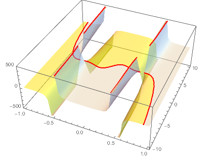
Here's a view of the discontinuities, rotated by Pi/4.

Plot3D[p - (1 + (0.2` (1 + 3 (p - q)^2))/(1 - (p - q)^2)^3) q /. {p ->
     x + y, q -> -x + y}, {x, -1, 1}, {y, -10, 10}, PlotPoints -> 51, 
 MaxRecursion -> 3, MeshFunctions -> {#3 &}, Mesh -> {{0}}, 
 MeshStyle -> {Thick, Red}, PlotStyle -> Opacity[0.5], 
 MeshShading -> {Directive[Opacity[0.5], Yellow], 
   Directive[Opacity[0.5], LightBlue]}, BoundaryStyle -> None, 
 Exclusions -> {1 - (p - q)^2 == 0 /. {p -> x + y, q -> -x + y}}, 
 PlotRange -> 500]

---

Responses to comments:

(1) One may get rid of the gaps introduced by the Exclusions option by plotting where the numerator (of the fraction resulting from Together):

ContourPlot[
 Evaluate@Thread[Numerator@Together[fulltable /. Equal -> Subtract] == 0],
 {p, -10, 10}, {q, -10, 10}, PlotPoints -> plotpoints]

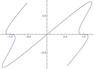
(2) Forgive me, but I'm not sure I understand the distinction between limiting range of a parameter in a parametric plot and limiting the plot range. Below is a parametric plot of the wiggly contour. Is that what you want? (Note the errors are unimportant, because that's what happens when the parametric solution heads towards infinity.)

fn = First@Numerator@Together@Union[Flatten[table5] /. Equal -> Subtract]
sol = NDSolve[{{p'[t], q'[t]} == (Cross[D[fn, {{p, q}}]] /. {p -> p[t], q -> q[t]}),
     {p[0], q[0]} == {0, 0}}, {p, q}, {t, -4, 4}]
(*
  -1. p + 3. p^3 - 3. p^5 + p^7 + 1.2 q - 8.4 p^2 q + 15. p^4 q - 
   7. p^6 q + 7.8 p q^2 - 30. p^3 q^2 + 21. p^5 q^2 - 2.4 q^3 + 
   30. p^2 q^3 - 35. p^4 q^3 - 15. p q^4 + 35. p^3 q^4 + 3. q^5 - 
   21. p^2 q^5 + 7. p q^6 - 1. q^7
*)

NDSolve::mxst: Maximum number of 10000 steps reached at the point t == -3.9211. >> NDSolve::mxst: Maximum number of 10000 steps reached at the point t == 3.921095435807773`. >>

{{p->InterpolatingFunction[{{-3.9211,3.9211}},<>],
  q->InterpolatingFunction[{{-3.9211,3.9211}},<>]}}

ParametricPlot[{p[t], q[t]} /. sol // Evaluate, {t, -3.4, 3.4}]

Answer 2

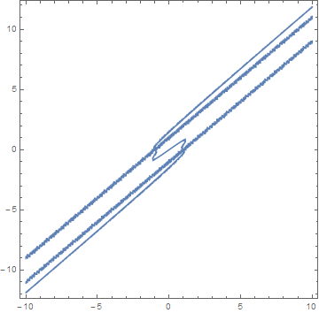
ContourPlot[
 p == q (1 + (2 (1 + 3 (p - q)^2) (.1))/(1 - (p - q)^2)^3), {p, -10, 
  10}, {q, -100, 100}, PlotPoints -> 150, PlotRange -> All, 
 Exclusions -> True]

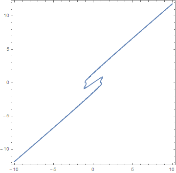
It seems to be the division in your expression that's giving you problems. Multiplying by (1 - (p - q)^2)^3 on both sides gives us:

ContourPlot[
 p (1 - (p - q)^2)^3 == 
  q ((1 - (p - q)^2)^3 + (2 (1 + 3 (p - q)^2) (.1))), {p, -10, 
  10}, {q, -100, 100}, PlotPoints -> 150, PlotRange -> All, 
 Exclusions -> True]

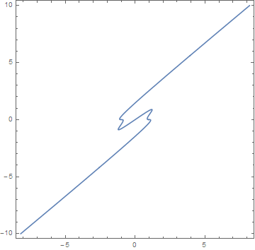
The remaining bit of fuzzyness comes from the fact that your range for q is too large: it goes from -100 to 100 when the actual range in the plot is more like -11 to +11. Setting the range to something more reasonable gives us:

ContourPlot[
 p (1 - (p - q)^2)^3 == 
  q ((1 - (p - q)^2)^3 + (2 (1 + 3 (p - q)^2) (.1))), {p, -10, 
  10}, {q, -10, 10}, PlotPoints -> 150, PlotRange -> All, 
 Exclusions -> True]

The reason the plot was stretched to the point where it looked bad was that you set PlotRange -> All, which zooms in to cover only the plotted points, even if they cover only a fraction of the range the plot was computed for. For a ContourPlot where you have already explicitly set the range this option is unnecessary, and can conceal range problems like this. In fact, the only option you need is MaxRecursion -> 3, since none of the features of the graph are small enough to be missed at the default PlotPoints setting.

ContourPlot[
 p (1 - (p - q)^2)^3 == 
  q ((1 - (p - q)^2)^3 + (2 (1 + 3 (p - q)^2) (.1))), {p, -10, 
  10}, {q, -10, 10}, MaxRecursion -> 3]

---

Note that this equation becomes greatly simplified when you rotate your coordinate system 45 degrees with the transformation

$$ u = \frac{p-q}{\sqrt{2}} \\ v = \frac{p+q}{\sqrt{2}} $$

Applying this to your original equation:

Simplify[Rationalize[
   p == q (1 + (2 (1 + 
            3 (p - q)^2) (.1))/(1 - (p - q)^2)^3)] /. {p -> (u + v)/
     Sqrt[2], q -> (v - u)/Sqrt[2]}]

$$ \frac{80 u^7-120 u^5+54 u^3+6 u^2 v-11 u+v}{2 u^2-1}=0 $$

This is trivially solved for $v$:

Simplify[Solve[%, v]]

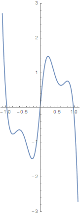
$$ v=\frac{-80 u^7+120 u^5-54 u^3+11 u}{6 u^2+1} $$

And plotted:

Plot[v /. %, {u, -1.1, +1.1}, AspectRatio -> Automatic]

Note that you can use ParametricPlot to display the solution in the original p, q coordinates.