Roots of Whittaker W function

Question

I am interested in finding the roots $u$ of the equation $$ W_{1,\imath b}(a)=0, $$ where $W_{\kappa,\mu}(z)$ denotes the Whittaker $W$ function, $a>0$ is a fixed parameter, $\imath=\sqrt{-1}$ and $b$ is the unknown. Due symmetry of the Whittaker $W$ with respect to $\mu$, it suffices to consider the above equation only for $b>0$. For any given $a>0$ the equation has countably many solutions, so numerically there is this issue of somehow telling Mathematica to ignore the solution it has already found.

I've written the following script

ClearAll[Evaluate[Context[] <> "*"]];

ϕ[x_, α_] := N[WhittakerW[1, (I α)/2, x]];
Subscript[α, opt][a_, β_] := α /. 
   FindRoot[ϕ[a, α], {α, β}];

a = 10;
β = 0;
For[i = 1, i <= 10, i += 1,
 β = 
  Subscript[α, opt][
   a, β*1.1]; (*tweak the starting point a bit so as to force \
Mathematica to look for zeros to the right of the previous one*)
 Print["a=", a, 
  ", \!\(\*SubscriptBox[\(α\), \(opt\)]\)=", β, 
  ", ϕ[a,\!\(\*SubscriptBox[\(α\), \(opt\)]\)]=", ϕ[
   a, β]];
 ]

I doubt though that the solutions the script outputs are correct. One issue is that they all have a nonzero imaginary component. Any suggestions as to how to improve the script?

Answer 1

This is a good example of the "dynamic range" problem in Boyd's CPR method (see also this answer by J.M.). As α moves toward -100, the OP's oscillatory Whittaker function decays exponentially. According to Boyd, where $ε_{mach}$ is the machine epsilon and $f_{max}$ is the maximum of $f(x)$ over an interval $[a,b]$, "If a function $f(x)$ has a magnitude as small as $|f (x)| \le O(ε_{mach}\, f_{max})$ on a subinterval within $[a,b]$ (excluding tiny subintervals around a zero), then $f(x)$ has, to borrow a term from photography, a large dynamic range." This can lead to numerical problems since the Chebyshev polynomials oscillate between ±1 throughout the interval. A Chebyshev series that is computed with floating-point numbers may have trouble representing a range greater than $ε_{mach}\, f_{max}$ to $f_{max}$. This is negligible if $f(x)$ passes quickly through the range $\pm ε_{mach}\, f_{max}$, such as near a zero of $f(x)$. There are two approaches to dealing with this issue. One can scale the function to alleviate the dynamic range, or one can subdivide the interval and find the roots piece-wise. We will show the scaling approach. The piecewise approach is feasible (with a interval length of 10 and WorkingPrecision -> 40), but we will show the scaling approach, which seems particularly appropriate here.

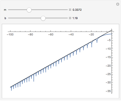
From the plot below, we can see that the rate of exponential decay is approximately

k = Rationalize[Log[10^0.3372], 0.01]
(*  7/9  *)

plot = Plot[RealExponent@WhittakerW[1, (I a)/2, 10], {a, -100, 0}, PlotPoints -> 100];
Manipulate[
 Show[
  plot,
  Graphics[{Dynamic[Line[{{0, b}, {-100, -100 m + b}}]]}]],
 {m, 0, 1, Appearance -> "Labeled"}, {b, 0, 2, Appearance -> "Labeled"}]

Alternatively, we can estimate the decay rate numerically from two distant peaks:

{m1, a1} = FindMaximum[Re@WhittakerW[1, (I a)/2, 10], {a, -40., -39.9}];
{m2, a2} = FindMaximum[Re@WhittakerW[1, (I a)/2, 10], {a, -100., -99.9}];
k = Rationalize[Log[m1/m2]/Subtract @@ (a /. {a1, a2}), 0.01]
(*  7/9  *)

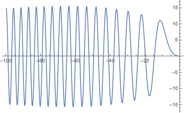
We can scale the Whittaker function to have a fairly even variation over the interval {-100, 0}.

Plot[Exp[-k α] WhittakerW[1, (I α)/2, 10], {α, -100, 0}, 
 WorkingPrecision -> 20, PlotRange -> All]

The function adaptiveChebSeries computes a Chebyshev series of a function $f(x)$ over $a \le x \le b$ to a given precision goal. The series $\sum c_j \, T_j(w)$ is in terms of $w = (2x - (a+b))/(b-a)$, where $-1 \le w \le 1$ for $a \le x \le b$. One can then compute companion matrix of the series, sometimes called the "colleague matrix," whose eigenvalues $w_j$ are the roots of the Chebyshev series. The roots $x_j$ of $f(x)$ will be the rescaled eigenvalues $x_j = ((b-a)w_j/2+(a+b)/2)$. The eigenvalues often have

(a0 = -100; b0 = 0;
  coeff = adaptiveChebSeries[                 (* get Chebyshev coefficients *)
    Exp[-k #] WhittakerW[1, (I #)/2, 10] &,
    a0, b0, PrecisionGoal -> 14.7];
  eigs = Eigenvalues@colleagueMatrix[coeff];  (* eigenvals of matrix contain the roots *)
  seeds = Sort@Rescale[                       (* select roots in [-1, 1] and *)
     Re@Select[                               (* rescale to [a0, b0] *)
       eigs,
       Abs[Im[#]] < 1*^-15 && -1.0001 < Re[#] < 1.0001 &],
     {-1, 1}, {a0, b0}];) // AbsoluteTiming
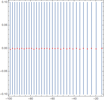
Length[seeds]

Eigenvalues::arh: Because finding 126 out of the 126 eigenvalues and/or eigenvectors is likely to be faster with dense matrix methods, the sparse input matrix will be converted. If fewer eigenvalues and/or eigenvectors would be sufficient, consider restricting this number using the second argument to Eigenvalues. >>

(*
  {0.87655, Null}
  32
*)

The last coefficient gives an estimate of the error bound.

Abs@Last@coeff
(*  6.80667*10^-15  *)

One can polish the eigenvalue-roots with FindRoot.

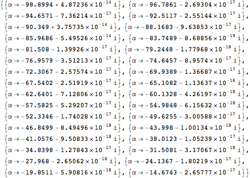
roots = α /. FindRoot[WhittakerW[1, (I α)/2, 10], {α, #}] & /@ seeds; // AbsoluteTiming
(*  {1.44508, Null}  *)

The seeds are pretty close to the roots. The residuals of the seeds and the roots are appropriately small.

(seeds - roots)/roots // Abs // Max
WhittakerW[1, (I roots)/2, 10] // Abs // Max
WhittakerW[1, (I seeds)/2, 10] // Abs // Max
(*
  3.54593*10^-15
  9.20479*10^-21
  1.09484*10^-18
*)

Since the Whittaker function has a fairly regular exponential decay, scaling by Exp[-k x] will give an approximate idea of the relative accuracy of the roots.

Exp[-k roots] WhittakerW[1, (I roots)/2, 10] // Abs // Max
Exp[-k seeds] WhittakerW[1, (I seeds)/2, 10] // Abs // Max
(*
  1.47868*10^-13
  6.84676*10^-12
*)

Code dump

The error in a Chebyshev series $\sum_{j=0}^N c_n T_n(x)$ for an analytic function is bounded by $\sum_{n > N} |c_n|$ and approximately equal to $|c_{N+1}| \le |c_{N}|$ if the series converges geometrically (or exponentially) and rapidly, since $|T_n(x)| \le 1$ for $-1 \le x \le 1$. If the function is analytic in a complex neighborhood of the interval $[-1,1]$, then the series will eventually converge geometrically. The coefficients are not guaranteed to decrease monotonically. For instance the Chebyshev polynomials are either even or odd functions, so for an even or odd function $f(x)$, every other Chebyshev coefficient will be zero. To help protect against mistakenly underestimating the error in such cases, we estimate the error by summing at least two terms of the tail of a series. Of course it is still possible for a function to be orthogonal to any number of successive Chebyshev polynomials, so such an error estimate can sometimes be fooled.

(* Chebyshev extreme points *)
chx[n_, prec_: MachinePrecision] := N[Cos[Range[0, n]/n Pi], prec];

(* Chebyshev series approximation to f *)
Clear[chebSeries];
chebSeries[f_, a_, b_, n_, prec_: MachinePrecision] := Module[{x, y, cc},
   x = Rescale[chx[n, prec], {-1, 1}, {a, b}];
   y = f /@ x; (* function values at Chebyshev points *)

   cc = Sqrt[2/n] FourierDCT[y, 1]; (* get coeffs from values *)

   cc[[{1, -1}]] /= 2;  (* adjust first & last coeffs *)
   cc
   ];

(* recursively double the Chebyshev points 
* until the PrecisionGoal is met 
* The function values are memoized in f0
* *)
Clear[adaptiveChebSeries];
Options[adaptiveChebSeries] = {PrecisionGoal -> 14, "Points" -> 32, 
   WorkingPrecision -> MachinePrecision, MaxIterations -> 5};
adaptiveChebSeries[f_, a_, b_, OptionsPattern[]] := 
 Module[{cc, f0, max, len = 0, sum},
  f0[x_] := f0[x] = f[x]; (* values reused in subsequent series *)
  NestWhile[
   (cc = chebSeries[f0, a, b, #, OptionValue[WorkingPrecision]];
     (* check error estimate *)
     max = Max@Abs@cc;   (* 
     sum the tail of the series *)
     sum = 0;            (* relative to the max coefficient *)
     len = LengthWhile[
       Reverse@cc, (sum += Abs@#) < 10^-OptionValue[PrecisionGoal]*max &];
     2 #) &,  (* double the number of points *)
   OptionValue["Points"],
   len < 2 && # <= 2^OptionValue[MaxIterations] OptionValue["Points"] &     (* 
   at least two coefficients dropped *)
   ];
  If[len < 2, 
   Message[adaptiveChebSeries::cvmit, OptionValue[MaxIterations]]];
  Drop[cc, -len]
  ]

(* "Chebyshev companion matrix" (Boyd, 2014) /
   "Colleague matrix" (Good, 1961) *)
colleagueMatrix[cc_] := With[{n = Length[cc] - 1},
   SparseArray[{{i_, j_} /; i == j + 1 :> 1/2, {i_, j_} /; i + 1 == j :> 
       1/(2 - Boole[i == 1])}, {n, n}] - 
    SparseArray[{{n, i_} :> cc[[i]]/(2 cc[[n + 1]])}, {n, n}]
   ];

Answer 2

You can use a plot to find the roots and then follow up with FindRoot to get precise solutions. Here I'll use ContourPlot to plot where the real part vanishes and use MeshFunctions to find where the imaginary part is simultaneously zero.

cp = Show[
  Table[
   ContourPlot[
    Evaluate[Re[WhittakerW[1, (I α)/2, 10] /. α -> a + b I] == 0],
    {a, a1, a1 + 10}, {b, -0.1, 0.1},
    PlotPoints -> {21, 5}, Mesh -> {{0}}, 
    MeshFunctions -> Function[{a, b}, Im[WhittakerW[1, (I α)/2, 10] /. α -> a + b I]],
     MeshStyle -> Red],
   {a1, -100, -10, 10}],
  PlotRange -> All]

seeds = Sort@Cases[Normal@cp, Point[p_] :> p, Infinity];
seeds // Short[#, 3] &
(*  {{-98.9014,-0.0024671},<<30>>,{-14.6835,-1.11492*10^-7}}  *)

FindRoot[WhittakerW[1, (I α)/2, 10], {α, #[[1]]}] & /@ seeds

To verify that the imaginary parts do vanish, increase WorkingPrecision:

FindRoot[WhittakerW[1, (I α)/2, 10], {α, #[[1]]},
 WorkingPrecision -> 30] & /@ seeds