30
$\begingroup$

It is common that I search numerically for all zeros (roots) of a function in a given range. I have written two simple minded functions that perform this task, and I know of similar functions on this site (e.g. this, this, and this).

I think this community will benefit if we could compile a list of functions that do so, with some explanations about efficiency considerations, in what context should we use which approach, etc.

The problem definition: given a function f and a range {x1,x2}, write a function that finds all (or most) roots of f in the given range.

$\endgroup$
6
  • 1
    $\begingroup$ The answer depends on how f is represented. Is it a pure black box, or is it possible to do exact operations on it (to, as a random example, factor out found roots). Can we take its derivatives? Can we assume it is defined outside of Interval[{x1,x2}], perhaps out onto some open set of the Complexes? $\endgroup$ Commented Aug 18, 2015 at 3:23
  • $\begingroup$ @EricTowers Good questions. The purpose of this post is to compile a list of answers that will suit different situations. If you have a solution that applies only to a few cases, please post it. $\endgroup$
    – yohbs
    Commented Aug 18, 2015 at 9:29
  • 2
    $\begingroup$ Er... have you guys ever seen this? library.wolfram.com/infocenter/Demos/4482 (Back in the days, Ted Ersek's RootSearch was all the rage on MathGroup) - Yeah, I know, it will come up it has been used below somewhere and I did not pay enough attention...) $\endgroup$
    – Peltio
    Commented Aug 21, 2015 at 8:04
  • $\begingroup$ @Peltio, yeah I remember that… now I'm wondering which of RootSearch[] or Wagon's FindAllCrossings[] came first. $\endgroup$ Commented Aug 21, 2015 at 13:54
  • $\begingroup$ @J.M. I wonder whether I should accept one of the answers or not. There's really no "correct answer" here, and this kind of a community wiki question. $\endgroup$
    – yohbs
    Commented Aug 27, 2015 at 7:27

4 Answers 4

22
$\begingroup$

First, it might be worth pointing out that in recent versions of Mathematica, Solve and NSolve are quite strong at solving equations with standard special functions.

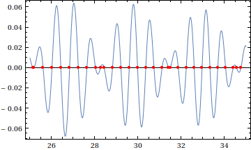
With[{f = BesselJ[1, #^(3/2)] Sin[#] &},
  solvesol = x /. Solve[{f[x] == 0, 25 <= x <= 35}, x];
  Plot[f[x], {x, 25, 35},
   MeshFunctions -> {# &}, Mesh -> {solvesol}, 
   MeshStyle -> Directive[PointSize[Medium], Red]
   ]
  ]

Solve::nint: Warning: Solve used numeric integration to show that the solution set found is complete. >>

Mathematica graphics


For other functions, provided they are continuous and not too oscillatory, then in addition to ODE approach in yohbs's NDSolve solution, we can solve the system with a DAE that does not need the function to be differentiable.

ClearAll[NrootSearch2];

Options[NrootSearch2] = Options[NDSolve];
NrootSearch2[f_, x1_, x2_, opts : OptionsPattern[]] := 
  Module[{x, y, t, s},
   Reap[
     NDSolve[{x'[t] == 1, x[x1] == x1, y[t] == f[t],
       WhenEvent[y[t] == 0, Sow[s /. FindRoot[f[s], {s, t}],
         "zero"],
        "LocationMethod" -> "LinearInterpolation"]},
      {}, {t, x1, x2}, opts],
     "zero"][[2, 1]]];

With[{f = BesselJ[1, #^(3/2)] Sin[#] &},
 nrootsol = NrootSearch2[f, 25, 35];
 Plot[f[x], {x, 25, 35},
  MeshFunctions -> {# &}, Mesh -> {nrootsol}, 
  MeshStyle -> Directive[PointSize[Medium], Red]
  ]
 ]

For functions like the example we've been using, we can combine the previous method with Root to produce exact results. (Caveat: Managing the precision of the approximate root is not always straightforward. Adjusting the WorkingPrecision option to FindRoot might be necessary. The code below tries it first at $MachinePrecision, and if that fails, then it tries a WorkingPrecision of 40.)

ClearAll[rootSearch2];

Options[rootSearch2] = Options[NDSolve];
rootSearch2[f_, x1_, x2_, opts : OptionsPattern[]] := 
  Module[{x, y, t, s, res, tmp},
   Reap[
     NDSolve[{x'[t] == 1, x[x1] == x1, y[t] == f[t],
       WhenEvent[y[t] == 0,
        Sow[Quiet[
          res = Check[
            Root[{f[#] &, 
              s /. FindRoot[f[s], {s, t}, WorkingPrecision -> $MachinePrecision]}],
        $Failed]];
         If[res === $Failed,  (* if $MachinePrecision fails, try a higher one *)
          Quiet[
           res = Check[
             Root[{f[#] &, 
               tmp = s /. 
                 FindRoot[f[s], {s, t}, WorkingPrecision -> 40]}],
             res = tmp]]];   (* if both fail, return approximate root *)
         res,
         "zero"],
        "LocationMethod" -> "LinearInterpolation"]},
      {}, {t, x1, x2}, opts],
     "zero"][[2, 1]]];

Note it returns 8 π etc. for the roots of the sine factor:

With[{f = BesselJ[1, #^(3/2)] Sin[#] &},
 exactsol = rootSearch2[f, 25, 35]
 ]
(*
  {8 π, 
   Root[{BesselJ[1, #1^(3/2)] Sin[#1] &, 
     25.192448602298225837336093255176323600186894730 + 0.*10^-46 I}], 
   Root[{BesselJ[1, #1^(3/2)] Sin[#1] &, 25.60802500579825}], 
   ...,
   11 π, 
   Root[{BesselJ[1, #1^(3/2)] Sin[#1] &, 34.76570243333289}]}
*)

Comparisons:

The two exact methods:

SortBy[N]@solvesol - exactsol // N[#, $MachinePrecision] &

N::meprec: Internal precision limit $MaxExtraPrecision = 50.` reached while evaluating {0,<<28>>,0}. >>

(*
{0, 0.*10^-65, 0, 0, 0, 0, 0, 0, 0, 0, 0, 0, 0, 0, 0, 0, 0, 0, 0, 0, 
0, 0, 0, 0, 0, 0, 0, 0, 0, 0}
*)

The two root-search methods:

nrootsol - N@exactsol
Max@Abs[%]
(*
  {0., 4.79616*10^-13, 3.55271*10^-15, 0., 0., 0., 0., 0., 0., -1.84741*10^-13, 
   2.8777*10^-13, 0., 0., 0., 0., 0., -3.55271*10^-15, 0., 0., 3.01981*10^-13, 0., 0., 0.,
   0., 0., 0., 7.10543*10^-15, -5.96856*10^-13, 7.10543*10^-15, 0.}

  5.96856*10^-13
*)
$\endgroup$
23
+100
$\begingroup$

One approach I've started to become fond of, apart from Plot[]-based approaches, involves the Chebyshev expansion of a function, followed by the construction of the corresponding "colleague matrix" (a matrix whose characteristic polynomial is the Chebyshev series previously determined), and then the computation of the colleague matrix's eigenvalues, which are hopefully good root approximations (perhaps followed by a polishing with FindRoot[] if wanted). The method is discussed in more detail in Boyd's book.

Using yohbs's example:

f = BesselJ[1, #^(3/2)] Sin[#] &; {xmin, xmax} = {25, 35};
n = 64;
cnodes = Rescale[N[Cos[Pi Range[0, n]/n], 20], {-1, 1}, {xmin, xmax}];
cc = Sqrt[2/n] FourierDCT[f /@ cnodes, 1];
cc[[{1, -1}]] /= 2;

colleague = SparseArray[{{i_, j_} /; i + 1 == j :> 1/2,
                         {i_, j_} /; i == j + 1 :> 1/(2 - Boole[j == 1])},
                        {n, n}] -
            SparseArray[{{i_, n} :> cc[[i]]/(2 cc[[n + 1]])}, {n, n}];

rts = Sort[Select[DeleteCases[
           Rescale[Eigenvalues[colleague], {-1, 1}, {xmin, xmax}],
                   _Complex | _DirectedInfinity], xmin <= # <= xmax &]];

Plot[f[x], {x, xmin, xmax},
     Epilog -> {Directive[Red, PointSize[Medium]], 
                Point[Transpose[PadRight[{rts}, {2, Automatic}]]]}]

oh hey, roots!

A more sophisticated approach which automatically chooses the number of sample points (in the style of Clenshaw-Curtis quadrature) is used in the MATLAB package Chebfun; as it is a bit more elaborate, I haven't gotten around to implementing it. Maybe one of these days...

$\endgroup$
7
  • $\begingroup$ Very interesting! You got a mix-up in the naming: comrade should be colleague in the expression for rts. Actually, maybe one should call it companion. $\endgroup$
    – Jens
    Commented Aug 21, 2015 at 5:46
  • 1
    $\begingroup$ @Jens, whoops yes. Mixed it up. Anyway: "companion" is quite general, "Frobenius companion" is the customary, well-known one, "comrade" refers to an orthogonal polynomial basis, and "colleague" is a Chebyshev comrade matrix. I felt out of breath just typing that… :D $\endgroup$ Commented Aug 21, 2015 at 5:54
  • $\begingroup$ J.M Would you tell me which font(Namely, the font of ticks 0.06, 0.04, 0.02,..) do you used in your graphic? $\endgroup$
    – xyz
    Commented Aug 21, 2015 at 6:07
  • 1
    $\begingroup$ @ShutaoTang Try adding the options ,PlotTheme->"Classic",Frame->True to Plot. $\endgroup$
    – Jens
    Commented Aug 21, 2015 at 6:09
  • $\begingroup$ I should probably stress this: compared to the functionality of MATLAB's chebfun, this is very primitive. It might take me a while to come up with working code for automatically choosing n. $\endgroup$ Commented Aug 22, 2015 at 6:56
18
$\begingroup$

The first approach is to evaluate the function at equidistant points, and look for sign changes. The distance between two sampled points, dx, is an input to the function. When a sign change happens, use FindRoot, which is constrained to look for the root only between the two points that encompass the sign change. The function accepts all the Options that FindRoot accepts.

rootSearch[f_, x1_, x2_, dx_, ops : OptionsPattern[]] := 
  Block[{xs, fs, fsb, pos},
   xs = Range[x1, x2, dx];
   fs = f /@ xs;
   fsb = Thread[fs > 0];
   pos = Flatten@Position[Thread[Xor[fsb // Rest, fsb // Most]], True];
   x /. ParallelTable[
     Quiet@
      FindRoot[
       f[x], {x, (xs[[p]] + xs[[p + 1]])/2, xs[[p]], xs[[p + 1]]}, 
       ops],
     {p, pos}]
   ];
Options[rootSearch] = Options[FindRoot]

This approach relies on knowing the adequate dx in advance. Setting it too low might result in slower computation, setting it too high might result in missing some roots.

The second approach does not have this caveat. It uses the built-in adaptive-mesh algorithms of NDSolve. The idea is to solve a differential equation that follows f, and look for sign changes. The function, rootSearchD, accepts all the Options of NDSolve.

rootSearchD[f_, x1_, x2_, ops : OptionsPattern[]] := Block[{fp, f1},
   fp = Derivative[1][f];
   f1 = f[x1];
   Last[Last[Reap[
      NDSolve[{y'[x$] == fp[x$], y[x1] == f1,
        WhenEvent[y[x$] == 0, Sow[x$]]}, y, {x$, x1, x2}, ops]
      ]]]
   ];
Options[rootSearchD] = Options[NDSolve];

A simple verification:

rootSearchD[Sin[#] &, 10, 20]/Pi
rootSearch[Sin[#] &, 10, 20, 1]/Pi

(*Output: {4., 5., 6.}*)

A more challenging example:

SetOptions[Plot, ImageSize -> 300, Axes -> {True, False}];
With[{f = BesselJ[1, #^(3/2) ] Sin[#] &},
 x1 = rootSearch[f, 25, 35, 0.1];
 x2 = rootSearchD[f, 25, 35];
 GraphicsRow@{
   Plot[f[x], {x, 25, 35}, 
    Epilog -> {Red, PointSize[Medium], Point[Transpose[{x1, 0 x1}]]}],
   Plot[f[x], {x, 25, 35}, 
    Epilog -> {Red, PointSize[Medium], Point[Transpose[{x2, 0 x2}]}]}
]

enter image description here

It is seen that rootSearch (the left panel) misses two roots that rootSearchD (the right panel) catches.

$\endgroup$
1
  • 1
    $\begingroup$ The alternative to equispaced sampling, as done in the first routine, is to use Plot[] for adaptive sampling; some of the routines linked to in the OP do this. $\endgroup$ Commented Aug 17, 2015 at 22:59
4
$\begingroup$

Don't forget the package RootSearch, it is the most robust root finding tool I have seen and fast. Since the package is quite old, directly running it has some warnings and some bugs. The author may update it these days.

I tried to realized a simplified and compact version of RootSearch using Mathematica built-in FindRoot and FindMinimum with suitable Accuracy and Precision Goal(without considering u function trick in RootSearch). I seems my version is already as robust as RootSearch as far as I test( But probably there are some vary rare cases that my version would fail while RootSearch will work. I don't know), and most of the time, my version is faster.

Any way, the basic idea behind my simplified RootSearch is three cases(credit to Ted Ersek)
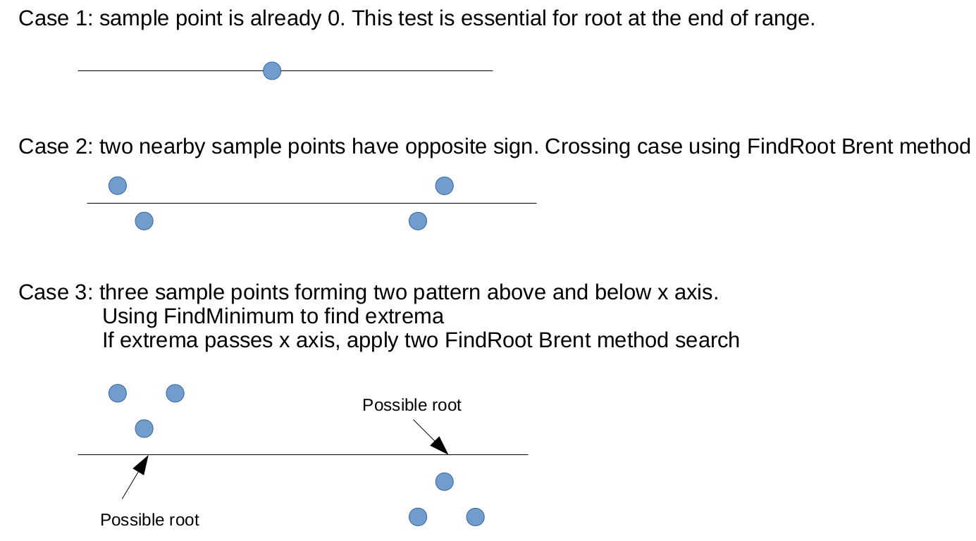
enter image description here

OK,Here is my version

ClearAll[myRootSearch];
Options[myRootSearch]={"samples"->150,"threshold"->10.^-10};
myRootSearch[f_,a_,b_,opts:OptionsPattern[{myRootSearch,FindRoot,FindMinimum}]]:=Module[{samples,threshold,rootByFindMinimum},
If[samples<2,Print["samples must be greater than 2. Aborted"];Abort[]];
samples=OptionValue["samples"];
threshold=OptionValue["threshold"];
xList=Subdivide[N@a,N@b,samples];
yList=f/@xList;
numericBool=NumericQ/@yList;
xList=Developer`ToPackedArray@Pick[xList,numericBool,True];
yList=Developer`ToPackedArray@N@Pick[yList,numericBool,True];
pointList=Transpose[{xList,yList}];

(*case 1: there are already some y are zeros. Especially handling roots at the two ends of range*)
zeroBool=Unitize[yList];
sol1=Pick[xList,zeroBool,0];

(*case 2: crossing x axis. Sign change occurs for two neighbor sample point. Brent method is suitable for crossing case*)
crossingPos=Flatten@Position[Sign[yList[[;;-2]]]*Sign[yList[[2;;]]],-1];
crossingIntervals=Transpose[{xList[[crossingPos]],xList[[crossingPos+1]]}];
roots=FindRoot[f[x],{x,#[[1]],#[[2]]},Method->"Brent",Evaluate@FilterRules[{opts},Options[FindRoot]],AccuracyGoal->10,PrecisionGoal->10]&/@crossingIntervals;
sol2=Flatten[roots][[;;,-1]];

(*case 3: three points concave downward to x asix, and three points convex upward to x axis*)
xListNoZero=Pick[xList,zeroBool,1];
yListNoZero=Pick[yList,zeroBool,1];
ratio1=1/Ratios[yListNoZero[[;;-2]]];
ratio2=Ratios[yListNoZero[[2;;]]];
ratio1Boole=1-UnitStep[1-ratio1];
ratio2Boole=1-UnitStep[1-ratio2];
turningPos=Flatten@Position[ratio1Boole*ratio2Boole,1];(*find where ratio1 and ratio2 are both greater than 1*)
turningIntervals=Transpose[{xListNoZero[[turningPos]],xListNoZero[[turningPos+2]]}];

If[Length@turningPos==0,
sol3={},
findExtremaWrapper[findExtremaFunc_,x0_,l_,r_]:=Module[{res,root,val,x},
newx0=If[x0==(l+r)/2.,x0+(r-x0)/10.^4,x0];
res=findExtremaFunc[f[x],{x,newx0,l,r},Method->"PrincipalAxis",Evaluate@FilterRules[{opts},Options[FindMinimum]],AccuracyGoal->10,PrecisionGoal->10];
val=First@res;
root=Last@Last@Last@res;
{root,val}];
roots=Table[
{left,middle,right}=xListNoZero[[i;;i+2]];
findExtremaFunc=If[yListNoZero[[i]]>0,FindMinimum,FindMaximum];
{root,val}=findExtremaWrapper[findExtremaFunc,middle,left,right];
(*if extrema pass x axis. apply additional two brent*)
If[(findExtremaFunc===FindMinimum&&val<0)||(findExtremaFunc===FindMaximum&&val>0),
{Last@Last@FindRoot[f[x],{x,left,root},Method->"Brent",Evaluate@FilterRules[{opts},Options[FindRoot]],AccuracyGoal->10,PrecisionGoal->10],
Last@Last@FindRoot[f[x],{x,root,right},Method->"Brent",Evaluate@FilterRules[{opts},Options[FindRoot]],AccuracyGoal->10,PrecisionGoal->10]},
root]
,{i,turningPos}];
sol3=Flatten@roots;
];
finalRoots=Select[DeleteDuplicates@Flatten[{sol1,sol2,sol3}],a<=#<=b&];
finalYList=f/@finalRoots;
finalPoints=Transpose[{finalRoots,finalYList}];
Select[finalPoints,Abs[Last[#]]<threshold&]
]

Now some benchmark.

Involve yohbs's rootSearch(change ParallelTable to Table for fair compare), rootSearchD, and FindAllCrossings

f = BesselJ[1, #^(3/2)] Sin[#] &;
{a, b} = {25, 35};
rootSearch[f, a, b, 0.1] // Length // RepeatedTiming
rootSearchD[f, a, b] // Length // RepeatedTiming
FindAllCrossings[f[x], {x, a, b}] // Length // RepeatedTiming
myRootSearch[f, a, b] // Length // RepeatedTiming

gives

{0.013, 26}

{0.021, 30}

{0.033, 30}

{0.00853, 30}

myRootSearch is fastest. If you check the root accuracy

In[156]:= f /@ rootSearchD[f, a, b]

Out[156]= {8.23994*10^-8, 7.6413*10^-8, 4.97188*10^-8, 4.77916*10^-8, 
 4.8088*10^-8, 4.07555*10^-8, 1.15119*10^-7, 6.35206*10^-8, 
 6.52786*10^-8, 5.79253*10^-8, 6.6591*10^-8, 7.52369*10^-8, 
 8.31748*10^-8, 7.03437*10^-8, 8.40684*10^-8, 8.26065*10^-8, 
 6.41365*10^-8, 
 2.00382*10^-8, -4.62283*10^-9, -3.48918*10^-9, -4.35917*10^-9, \
-2.76901*10^-8, -2.05933*10^-8, -2.27062*10^-8, -1.23489*10^-8, \
-2.05456*10^-8, 7.48906*10^-9, -4.0179*10^-9, 1.33413*10^-8, 
 1.5595*10^-8}

In[157]:= f /@ FindAllCrossings[f[x], {x, a, b}]

Out[157]= {3.02444*10^-17, -7.75062*10^-17, 8.55344*10^-16, 
 5.62506*10^-16, 8.2445*10^-16, 
 6.59322*10^-16, -1.15639*10^-13, -5.96458*10^-16, -2.68016*10^-15, 
 4.70709*10^-14, -4.35389*10^-16, -2.28363*10^-13, -9.36274*10^-14, 
 6.00381*10^-16, 1.79983*10^-14, -9.12193*10^-16, -2.88893*10^-13, 
 8.59057*10^-12, -2.07482*10^-13, -1.71217*10^-17, -2.00521*10^-16, \
-8.66952*10^-16, 1.38108*10^-15, -3.84904*10^-16, -2.01267*10^-14, 
 4.1645*10^-14, -4.85453*10^-13, 2.53398*10^-12, 
 5.25131*10^-15, -4.64579*10^-17}

In[158]:= f /@ myRootSearch[f, a, b][[;; , 1]]

Out[158]= {3.02444*10^-17, 4.28317*10^-17, -9.67757*10^-16, 5.62506*10^-16, 
8.2445*10^-16, 6.59322*10^-16, 
 2.21338*10^-15, -5.96458*10^-16, -2.97296*10^-17, -6.77043*10^-17, 
 1.31741*10^-16, -1.97586*10^-16, -2.14801*10^-15, 6.00381*10^-16, 
 4.5716*10^-16, 2.13891*10^-15, -7.06261*10^-16, 9.66224*10^-17, 
 4.31717*10^-17, -1.71217*10^-17, 5.29798*10^-16, -8.66952*10^-16, 
 1.38108*10^-15, -3.84904*10^-16, -1.13785*10^-16, -1.58097*10^-15, \
-5.33152*10^-16, 2.56233*10^-16, -1.19073*10^-16, -4.64579*10^-17}

myRootSearch is quite good.


challenge cases

the above example is not that challenge.

Now I define a show function

ClearAll[myRootSearchShow];
myRootSearchShow[f_, a_, b_, opts : OptionsPattern[]] := 
 Module[{points},
  roots = 
   myRootSearch[f, a, b, FilterRules[{opts}, Options[myRootSearch]]];
  roots = If[roots == {}, {}, roots[[;; , 1]]];
  points = {#, f[#]} & /@ roots;
  Plot[f[x], {x, a, b}, 
   Epilog -> {PointSize[Medium], Red, Point[points]}]]

and try this

f = Abs[Zeta[1/2 + I #]]&;
{a, b} = {0, 30};
rootSearchD[f, a, b] // Length // RepeatedTiming
FindAllCrossings[f[x], {x, a, b}] // Length // RepeatedTiming
myRootSearch[f, a, b] // Length // RepeatedTiming

gives

{0.00061, 1}

{0.028, 0}

{0.0053, 3}

rootSearchD prompt error, FindAllCrossings can not find any. The actual roots are very particular. It is handled by case 3, so that is why all other method are not working.

Run myRootSearchShow[f, a, b] shows
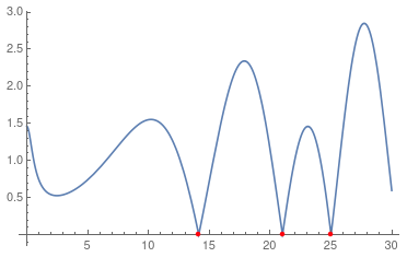
enter image description here

and pretty good accuracy

f /@ myRootSearch[f, a, b][[;; , 1]]
{4.36811*10^-15, 7.18232*10^-15, 6.5642*10^-15}

What about shift the curve down a little, there should be 6 roots.

f = (Abs[Zeta[1/2 + I #]] - 0.0001) &;
{a, b} = {0, 30};
rootSearchD[f, a, b] // Length // RepeatedTiming
FindAllCrossings[f[x], {x, a, b}] // Length // RepeatedTiming
myRootSearch[f, a, b] // Length // RepeatedTiming

it gives

{0.00061, 1}

{0.03, 0}

{0.00650, 6}

still only myRootSearch find all 6 roots. and

f /@ myRootSearch[f, a, b][[;; , 1]]
{-1.16174*10^-15, -1.1204*10^-15, 
 2.3646*10^-15, -1.95511*10^-15, -1.02109*10^-15, 3.65443*10^-15}

If the searching range is long or the function is oscillating so much , don't forget to set higher samples.

f = (-Abs[Zeta[1/2 + I #]]) &;
myRootSearchShow[f, 0, 100, "samples" -> 300]

gives
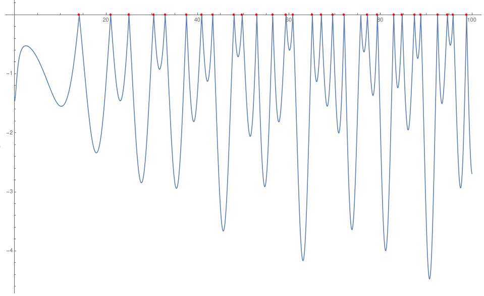
enter image description here

If function involves some singularities, myRootSearch may give some warning. Most of the time, it is harmless. For example

myRootSearch[Cot, 0, 2 Pi]

it gives

During evaluation of In[820]:= FindRoot::brmp: The root has been bracketed as closely as possible with machine precision but the function value exceeds the absolute tolerance 9.99999999999996`*^-11.

Out[820]= {{1.5708, 6.12323*10^-17}, {4.71239, 1.83697*10^-16}}

This is because, FindRoot can not find root around sigularity, because there is no root at all! But the result is perfectly right as you can see from
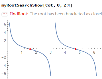
enter image description here

Anyway, you can always check the second element of each sublist of the result to make sure that function values at root position are indeed almost zero. In this case, they are 6.12323*10^-17 and 1.83697*10^-16.

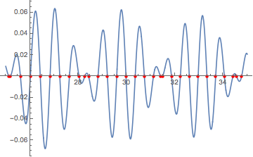
Finally, in case 3 it is the extrema that are sought. So there is a "threshold" option as a root filter. The default I set is somewhat loosely as 10^-10. If you set it as 10^-14,it means that function value must be smaller then 10^-14 to be considered as a root, all other "roots" are considered fake and discarded.

$\endgroup$

Your Answer

By clicking “Post Your Answer”, you agree to our terms of service and acknowledge you have read our privacy policy.

Not the answer you're looking for? Browse other questions tagged or ask your own question.