Bounty Ended with 100 reputation awarded by ciao
added 2 characters in body
Source Link

One approach I've started to become fond of, apart from Plot[]-based approaches, involves the Chebyshev expansion of a function, followed by the construction of the corresponding "colleague matrix" (a matrix whose characteristic polynomial is the Chebyshev series previously determined), and then the computation of the colleague matrix's eigenvalues, which are hopefully good root approximations (perhaps followed by a polishing with FindRoot[] if wanted). The method is discussed in more detail in Boyd's book.

Using yohbs's example:

f = BesselJ[1, #^(3/2)] Sin[#] &; {xmin, xmax} = {25, 35};
n = 64;
cnodes = Rescale[N[Cos[Pi Range[0, n]/n], 20], {-1, 1}, {xmin, xmax}];
cc = Sqrt[2/n] FourierDCT[f /@ cnodes, 1];
cc[[{1, -1}]] /= 2;

colleague = SparseArray[{{i_, j_} /; i + 1 == j :> 1/2,
                         {i_, j_} /; i == j + 1 :> 1/(2 - Boole[j == 1])},
                        {n, n}] -
            SparseArray[{{i_, n} :> cc[[i]]/(2 cc[[n + 1]])}, {n, n}];

rts = Sort[Select[DeleteCases[
           Rescale[Eigenvalues[comrade]Rescale[Eigenvalues[colleague], {-1, 1}, {xmin, xmax}],
                   _Complex | _DirectedInfinity], xmin <= # <= xmax &]];

Plot[f[x], {x, xmin, xmax},
     Epilog -> {Directive[Red, PointSize[Medium]], 
                Point[Transpose[PadRight[{rts}, {2, Automatic}]]]}]
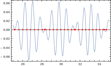
oh hey, roots!

A more sophisticated approach which automatically chooses the number of sample points (in the style of Clenshaw-Curtis quadrature) is used in the MATLAB package Chebfun; as it is a bit more elaborate, I haven't gotten around to implementing it. Maybe one of these days...

One approach I've started to become fond of, apart from Plot[]-based approaches, involves the Chebyshev expansion of a function, followed by the construction of the corresponding "colleague matrix" (a matrix whose characteristic polynomial is the Chebyshev series previously determined), and then the computation of the colleague matrix's eigenvalues, which are hopefully good root approximations (perhaps followed by a polishing with FindRoot[] if wanted). The method is discussed in more detail in Boyd's book.

Using yohbs's example:

f = BesselJ[1, #^(3/2)] Sin[#] &; {xmin, xmax} = {25, 35};
n = 64;
cnodes = Rescale[N[Cos[Pi Range[0, n]/n], 20], {-1, 1}, {xmin, xmax}];
cc = Sqrt[2/n] FourierDCT[f /@ cnodes, 1];
cc[[{1, -1}]] /= 2;

colleague = SparseArray[{{i_, j_} /; i + 1 == j :> 1/2,
                         {i_, j_} /; i == j + 1 :> 1/(2 - Boole[j == 1])},
                        {n, n}] -
            SparseArray[{{i_, n} :> cc[[i]]/(2 cc[[n + 1]])}, {n, n}];

rts = Sort[Select[DeleteCases[
           Rescale[Eigenvalues[comrade], {-1, 1}, {xmin, xmax}],
                   _Complex | _DirectedInfinity], xmin <= # <= xmax &]];

Plot[f[x], {x, xmin, xmax},
     Epilog -> {Directive[Red, PointSize[Medium]], 
                Point[Transpose[PadRight[{rts}, {2, Automatic}]]]}]

oh hey, roots!

A more sophisticated approach which automatically chooses the number of sample points (in the style of Clenshaw-Curtis quadrature) is used in the MATLAB package Chebfun; as it is a bit more elaborate, I haven't gotten around to implementing it. Maybe one of these days...

One approach I've started to become fond of, apart from Plot[]-based approaches, involves the Chebyshev expansion of a function, followed by the construction of the corresponding "colleague matrix" (a matrix whose characteristic polynomial is the Chebyshev series previously determined), and then the computation of the colleague matrix's eigenvalues, which are hopefully good root approximations (perhaps followed by a polishing with FindRoot[] if wanted). The method is discussed in more detail in Boyd's book.

Using yohbs's example:

f = BesselJ[1, #^(3/2)] Sin[#] &; {xmin, xmax} = {25, 35};
n = 64;
cnodes = Rescale[N[Cos[Pi Range[0, n]/n], 20], {-1, 1}, {xmin, xmax}];
cc = Sqrt[2/n] FourierDCT[f /@ cnodes, 1];
cc[[{1, -1}]] /= 2;

colleague = SparseArray[{{i_, j_} /; i + 1 == j :> 1/2,
                         {i_, j_} /; i == j + 1 :> 1/(2 - Boole[j == 1])},
                        {n, n}] -
            SparseArray[{{i_, n} :> cc[[i]]/(2 cc[[n + 1]])}, {n, n}];

rts = Sort[Select[DeleteCases[
           Rescale[Eigenvalues[colleague], {-1, 1}, {xmin, xmax}],
                   _Complex | _DirectedInfinity], xmin <= # <= xmax &]];

Plot[f[x], {x, xmin, xmax},
     Epilog -> {Directive[Red, PointSize[Medium]], 
                Point[Transpose[PadRight[{rts}, {2, Automatic}]]]}]

oh hey, roots!

A more sophisticated approach which automatically chooses the number of sample points (in the style of Clenshaw-Curtis quadrature) is used in the MATLAB package Chebfun; as it is a bit more elaborate, I haven't gotten around to implementing it. Maybe one of these days...

Source Link

One approach I've started to become fond of, apart from Plot[]-based approaches, involves the Chebyshev expansion of a function, followed by the construction of the corresponding "colleague matrix" (a matrix whose characteristic polynomial is the Chebyshev series previously determined), and then the computation of the colleague matrix's eigenvalues, which are hopefully good root approximations (perhaps followed by a polishing with FindRoot[] if wanted). The method is discussed in more detail in Boyd's book.

Using yohbs's example:

f = BesselJ[1, #^(3/2)] Sin[#] &; {xmin, xmax} = {25, 35};
n = 64;
cnodes = Rescale[N[Cos[Pi Range[0, n]/n], 20], {-1, 1}, {xmin, xmax}];
cc = Sqrt[2/n] FourierDCT[f /@ cnodes, 1];
cc[[{1, -1}]] /= 2;

colleague = SparseArray[{{i_, j_} /; i + 1 == j :> 1/2,
                         {i_, j_} /; i == j + 1 :> 1/(2 - Boole[j == 1])},
                        {n, n}] -
            SparseArray[{{i_, n} :> cc[[i]]/(2 cc[[n + 1]])}, {n, n}];

rts = Sort[Select[DeleteCases[
           Rescale[Eigenvalues[comrade], {-1, 1}, {xmin, xmax}],
                   _Complex | _DirectedInfinity], xmin <= # <= xmax &]];

Plot[f[x], {x, xmin, xmax},
     Epilog -> {Directive[Red, PointSize[Medium]], 
                Point[Transpose[PadRight[{rts}, {2, Automatic}]]]}]

oh hey, roots!

A more sophisticated approach which automatically chooses the number of sample points (in the style of Clenshaw-Curtis quadrature) is used in the MATLAB package Chebfun; as it is a bit more elaborate, I haven't gotten around to implementing it. Maybe one of these days...