Determine frequency of oscillations

Question

I am wondering how I could determine the frequency of oscillations of a differential model equation? How could I find the frequency from this example given in Mathematica Documentation:

s = NDSolve[{y'[x] == y[x] Cos[x + y[x]], y[0] == 1}, y, {x, 0, 30}]
Plot[Evaluate[y[x] /. s], {x, 0, 30}, PlotRange -> All]

I am asking because I need to determine the frequency of one model term as a function of a the strength of a second model term, in a much more complicated model than described above.

Answer 1

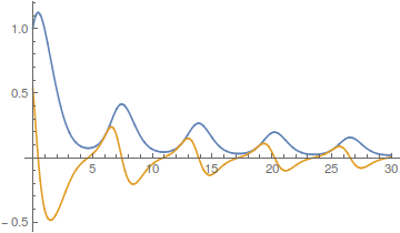
I'd advocate taking differences between successive peaks and likewise troughs. These can be found by keeping track of when the derivative is zero.

pts = 
 Reap[s = NDSolve[{y'[x] == y[x] Cos[x + y[x]], y[0] == 1, 
      WhenEvent[y'[x] == 0, Sow[x]]}, {y, y'}, {x, 0, 30}]][[2, 1]]

(* Out[290]= {0.448211158984, 4.6399193764, 7.44068279785, 10.953122261, \
13.8722260952, 17.2486864443, 20.2244048853, 23.5386505821, \
26.5478466115, 29.8261176372} *)

Plot[{Evaluate[y[x] /. s], Evaluate[y'[x] /. s]}, {x, 0, 30}, 
 PlotRange -> All]

diffs = Differences[pts, 1, 2]

(* Out[288]= {6.99247163887, 6.31320288463, 6.43154329733, \
6.29556418327, 6.35217879014, 6.28996413777, 6.32344172616, \
6.28746705515} *)

Mean[diffs]

(* Out[289]= 6.41072921417 *)

Noticing that the first might be an outlier, one might choose to discard it.

Mean[Rest[diffs]]

(* Out[291]= 6.32762315349 *)

Answer 2

The classical Fourier approach

Your data :

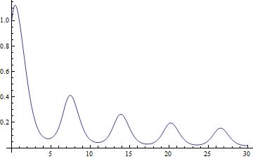
s = NDSolve[{y'[x] == y[x] Cos[x + y[x]], y[0] == 1}, y, {x, 0, 30}][[1, 1, 2]];
Plot[s[x], {x, 0, 30}, PlotRange -> All]

The horizontal axis is supposed to be graduated in seconds.
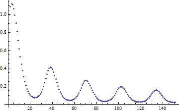
First, we sample s at the frequency 5 Hz :

data00 = s /@ Range[0, 30, 1/5];
ListLinePlot[data00, PlotRange -> All, PlotStyle -> Thick, Joined -> False]

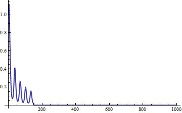
To increase the resolution of the Fourier transform, this record is extended to 1000 samples, so that the resolution of the fourier transform is fine enough (5/1000 = 5 mHz between each sample) :

data01 = PadRight[data00, 1000];
ListLinePlot[data01, PlotRange -> All, PlotStyle -> Thick]

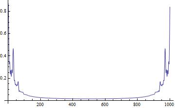
The spectrum is calculated :

data02 = Abs[Fourier[data01]];
ListLinePlot[data02, PlotRange -> All]

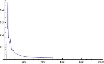
To localise precisely where is the peak near the coordinates {40, 0.45}, we reject the uninteresting frequencies. Then we look for the maximum with Ordering[] :

data03 = Table[If[20 < i < 500, data02[[i]], 0.], {i, Length[data02]}];
ListLinePlot[data03, PlotRange -> All] 
First[Ordering[data03, -1]] (* maximum *)

32

The peak is at position 32 on the horizontal axis. This means that the frequency is (32 - 1)*0.005 = 0.155Hz, that is to say period=6.45 second.

Answer 3

I'm not very good at Mathematica, but I think there are two "usual" ways of solving this problem.

One is to do a Fourier transform of your data, and find the peak. Unfortunately I couldn't get a result from Mathematica in a way that makes sense for this.

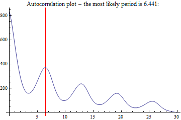
The other option is to use an autocorrelation plot, and take the best peak. I'm not sure how to do this for a function, but you can sample points along your function and then work with those points:

Let's input your data, and make a plot: (I won't include a plot here since you already have it in the question)

s = NDSolve[{y'[x] == y[x] Cos[x + y[x]], y[0] == 1}, y, {x, 0, 30}]; 
Plot[Evaluate[y[x] /. s], {x, 0, 30}, PlotRange -> All]

Sample the solution at 10.000 equally spaced points:

numPoints = 10000;
samplePoints = Range[0, 30, 30/numPoints];
samples = Evaluate[y[samplePoints] /. s][[1]];
ListPlot[samples]; (* You can plot the sampled points to be sure, but I disabled it *)

Calculate the autocorrelation:

autocorrelations = ListCorrelate[samples, samples , {1, 1}, 0];

Find peaks by looking for points where the differential changes sign:

peaks = 1 + Position[Differences[Sign[Differences[autocorrelations]]], -2];
bestPeriods = Extract[samplePoints, peaks];

Note that if you have Mathematica 9+, then the above code can be simplified to just MinDetect. See https://mathematica.stackexchange.com/a/19838/578

Create a nice plot of the autocorrelation, and draw a red line at the most likely peak:

xyPoints = Transpose[{samplePoints, autocorrelations}];
ListLinePlot[xyPoints, PlotRange -> All, GridLines -> {{{First[bestPeriods], Red}}, {}}, PlotLabel -> "Autocorrelation plot - the most likely period is " <> ToString[First[bestPeriods]] <> ":"]

If you want to use the detected period for something, you can access it with First[bestPeriods].