Another way to calculate frequency from Fourier transform

Question

I have some trouble with calculating frequency after Fourier transform. My code:

fB = 1.0;
TimeStart = 0;
TimeEnd = 5;
Data1 = Table[Sin[2 Pi fB x], {x, 0, 5, 1/10}];
sra = 10./1;
inco = sra/Length[Data1];
fresa = Table[f, {f, 0, sra - inco, inco}];
ListPlot[Transpose[{fresa, Flatten[Abs[Fourier[Data1]]]}], 
Joined -> True, Frame -> True, 
FrameLabel -> {Row[{Style["Frequency, (a.u.)", FontSlant -> Italic, 
FontSize -> 15]}], Row[{Style["Amplitude, (a.u.)", FontSlant -> Italic, 
FontSize -> 15]}]}, LabelStyle -> Blue, 
FrameTicksStyle -> Directive[Orange, 15], ImageSize -> 900, 
PlotStyle -> {Red}, Joined -> True, AspectRatio -> 0.5, 
PlotRange -> {All, All}, Epilog -> {PointSize[0.003], 
Point[Transpose[{fresa, Flatten[Abs[Fourier[Data1]]]}]]}]

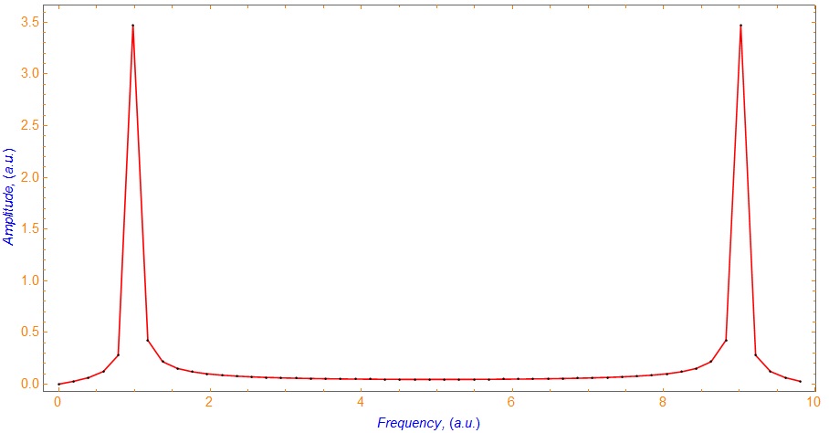
Result:

To find frequency I have next part of code:

Data21 = Flatten[Abs[Fourier[Data1]]];
Pos = Position[Data21, Max[Data21]][[1, 1]]
gf = (Pos - 1)/((TimeEnd - TimeStart))

result is:

1.0 Hz

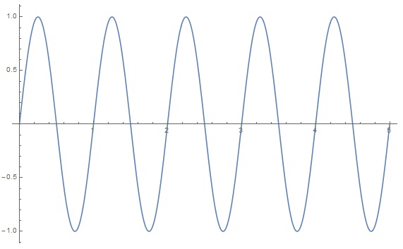
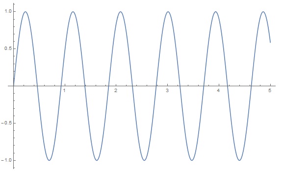
Is there any more accurate way to determine the frequency than the one above? Cause if we tried to change parametrs slowly, we don's see changing of frequency. For example if we change fB from 1.0 to 1.08. From sin graph we can see that frequency rises.

When fB = 1.0

When fB = 1.08

Programm calculate that frequency in both cases is 1 Hz.

Answer 1

There are two problems here :

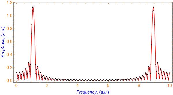
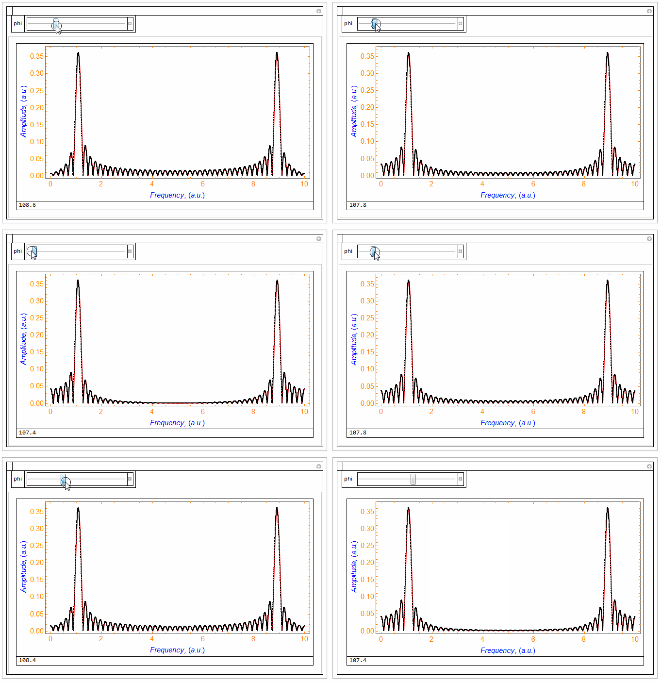
• Due to the fact that the duration of the acquisition is 5 seconds, the FFT has a resolution of 1/5 = 0.2Hz, that is to say, there is one point every 0.2Hz in the frequency domain. So you can't have something between 1Hz and 1.2Hz. A solution is to add padding, as explained here. With a padding of 501 one obtains this :

10.8 Hz

• Seems to be OK, but there is a second point: The value 10.8 Hz is not independent of the phase. With a padding of 5001 one obtains :

Here is the corresponding code :

Manipulate[
 fB = 1.08;
 TimeStart = 0;
 TimeEnd = 5;
 Data1 = PadRight[Table[Sin[2 Pi fB x + phi], {x, 0, 5, 1/10}], 5001];
 sra = 10./1;
 inco = sra/Length[Data1];
 fresa = Table[f, {f, 0, sra - inco, inco}];
 ListPlot[Transpose[{fresa, Flatten[Abs[Fourier[Data1]]]}], 
   Joined -> True, Frame -> True, 
   FrameLabel -> {Row[{Style["Frequency, (a.u.)", FontSlant -> Italic,
         FontSize -> 15]}], 
     Row[{Style["Amplitude, (a.u.)", FontSlant -> Italic, 
        FontSize -> 15]}]}, LabelStyle -> Blue, 
   FrameTicksStyle -> Directive[Orange, 15], ImageSize -> 600, 
   PlotStyle -> {Red}, Joined -> True, AspectRatio -> 0.5, 
   PlotRange -> {All, All}, 
   Epilog -> {PointSize[0.003], 
     Point[Transpose[{fresa, Flatten[Abs[Fourier[Data1]]]}]]}] //
  Column[{#
     , Data21 = Take[Flatten[Abs[Fourier[Data1]]], 2500];
     Pos = Position[Data21, Max[Data21]][[1, 1]];
     (Pos - 1)/((TimeEnd - TimeStart)) // N}] &,
 {{phi, 0}, 0, 2 Pi}]  

The origin of this phenomeon is that you have very few alternances of the sinus in your acquisition (5 alternances). If you can get a acquisition with more alternances this is the best way to go. Otherwise there are solutions to get 10.8 whatever the phase.

Answer 2

Try the following code where f is frequency.

test[f_, n_: 10, eps_: 1/30] := With[
  {sig = Table[Sin[2 Pi f x], {x, 0, 1, eps}]},
  Take[Drop[Fourier @ sig, 1], n]//Abs];
MatrixPlot @ Table[test[f, 10, 1/30], {f, 10}]

Notice the Take[Drop[..., 1], n]//Abs which extracts the strength of the frequencies from 1 to n.

In your code you have the frequencies too close together. In my code, the frequencies are well separated. As is documented, Fourier[] computes the Discrete Fourier Transform. It is designed to clearly distringuish a given frequency and its subharmonics.

Of course, you probably have some application in mind and have not stated what the real problem you are trying to solve is. It probably involves real world data with noise is my best guess.

Answer 3

Just for fun you can fit a 2nd order curve to the data around the peak and interpolate the actual peak. You have from your code, with a small mod to make sure we grab the first peak only:

data21 = Flatten[Abs[Fourier[Data1]]];
pos = Position[data21, Max[data21[[1 ;; Floor[Length[data21]/2]]]]][[1, 1]];
gf = (pos - 1)/((TimeEnd - TimeStart))

Now grab the points near the peak and do a 2nd order fit there

dr = Range[pos - 1, pos + 1]
subdat = Transpose[{dr, data21[[dr]]}]
posApprox = Solve[D[Fit[subdat, {1, x, x^2}, x], x] == 0] // Values // Flatten // First;
gff = (posApprox - 1)/((TimeEnd - TimeStart))

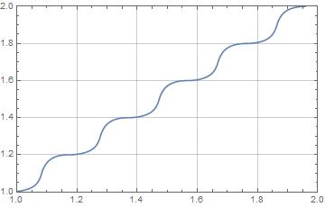
Plot a comparison as you vary fB, between gff and fB. Not hideously shabby. Could probably find a better fitting function for the peak.

res = Table[{fB,
   TimeStart = 0;
   TimeEnd = 5;
   Data1 = Table[Sin[2 Pi fB x], {x, 0, 5, 1/10}];
   sra = 10./1;
   inco = sra/Length[Data1];
   fresa = Table[f, {f, 0, sra - inco, inco}];
   data21 = Flatten[Abs[Fourier[Data1]]];
   pos = Position[data21, Max[data21[[1 ;; Floor[Length[data21]/2]]]]][[1, 1]];
   dr = Range[pos - 1, pos + 1];
   subdat = Transpose[{dr, data21[[dr]]}];
   posApprox = Solve[D[Fit[subdat, {1, x, x^2}, x], x] == 0] // Values //  Flatten // First;
   gff = (posApprox - 1)/((TimeEnd - TimeStart))}
  , {fB, 1, 2, .01}]