Data fitting with Image processing feature detection

Question

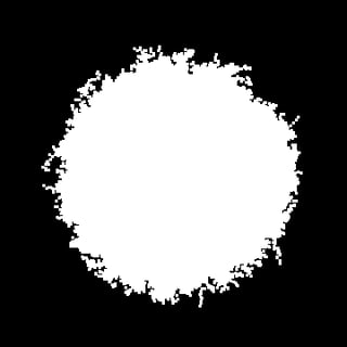
I have some 2D data that once plotted looks like the following

dat=Import["data.mat","Data"];
picList=ListPlot[,Axes-> None,Frame-> None,AspectRatio-> 1];
e=ColorConvert[Rasterize[picList],"Grayscale"];
Show[picList,Frame-> True]

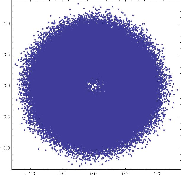
Now I wrote the following image processing function to detect the outer circular region where the point density starts to decrease. I want to fit that region with a certain parametric curve. For example a circle with unknown radius $r$. I want to achieve this through an automatic code without any manual input (one can use Manipulate with ListPlot for instance).

I have included extensive commenting for better understanding my approach for a solution.

The Function:

FinalFit[res_, TotalVariationFilter$Regularization_: .2, 
TotalVariationFilter$MaxIterations_: 10, 
GradientFilter$PixelRadius_: 1, BoundingBoxPoints_: 50, 
ExtraImage_: False] := 
Block[{picList, e, addedIm, Finres, dimX, dimY, imRange, plotrange, 
datim, res1, intData, finder, fun, xvals, yvals, boxdat, circledat,
arrow, Pic, r},
(*------ Take the 2D data points and plot it *)
picList = 
ListPlot[res, Axes -> None, Frame -> None, AspectRatio -> 1];
(*------ 
Create a raster image from the plot and convert it to Grayscale *)
e = ColorConvert[Rasterize[picList], "Grayscale"];
(*------ Reduce the noise in the outward part of the cluster *)
addedIm = 
ImageAdd[ 
 TotalVariationFilter[Binarize[e], 
  TotalVariationFilter$Regularization, 
  MaxIterations -> TotalVariationFilter$MaxIterations], e] // 
Binarize;
(*------ Get the ridges of gradient lines in the binarize image *)
Finres = (GradientFilter[addedIm, GradientFilter$PixelRadius, 
  "NonMaxSuppression" -> True] // Binarize);
(*------ Dimension of the input raster "e" *)
{dimX, dimY} = N[ImageDimensions@e];
imRange = {{1., dimX}, {1., dimY}};
(*------ Extract the 2D data range *)
plotrange = AbsoluteOptions[picList, PlotRange][[1]][[2]];
(*------ Get the image data from last image with gradient lines *)
datim = Reverse@ImageData[Finres];
res1 = Table[{i, j, N[datim[[i, j]]]}, {i, 1, dimX}, {j, 1, dimY}];
(*------ Rescale the contour/
gradient line according to the 2D data range "Bad Coding!" *)
intData = 
Join[Transpose@
  RescalingTransform[imRange, plotrange][
   Flatten[Table[{i, j}, {i, 1, dimX}, {j, 1, dimY}], 1]], {Last@
   Transpose@Flatten[res1, 1]}] // Transpose;
(*------ 
Form a Nearest function with the above obtained points constituting \
the target contour *)
(*------ Select the points on the contour as their third co-
ordinate correspond to the pixel value of "1." *)
finder = Nearest[Take[Select[intData, #[[3]] == 1. &], All, 2]];
(*------ 
On the contour line image discretize the boundary with uniformly \
seperated points *)
(*------ User specifies the number of total bounding points *)
(*------ Start of "Bad Codeing!" *)
xvals = 
Range[#[[1]], #[[2]], (#[[2]] - #[[1]])/(BoundingBoxPoints/
      4)] & /@ {plotrange[[1]]} // Flatten;
yvals = 
Range[#[[1]], #[[2]], (#[[2]] - #[[1]])/(BoundingBoxPoints/
      4)] & /@ {plotrange[[2]]} // Flatten;
boxdat = 
DeleteDuplicates@(Join[
  Join[Map[{#, yvals // First} &, xvals], 
   Map[{#, yvals // Last} &, xvals]], 
  Join[Map[{xvals // First, #} &, yvals], 
   Map[{xvals // Last, #} &, yvals]]]);
(*------ End of "Bad Codeing!" *)
(*------ Find the points on the quasi-
circular contour that is Nearest to the discrete boundary  *)
circledat = Map[First@finder[#] &, boxdat];
(*------ Start Visualization *)
arrow = 
Show[Flatten@
 MapThread[
  Graphics[{Thickness[.002], 
     Red, {Arrowheads[.02], Arrow[{#1, #2}]}}] &, {boxdat, 
   circledat}], Frame -> True]; 
Pic = Show[{arrow, 
 ListPlot[{boxdat, circledat[[FindCurvePath[circledat][[1]]]], 
   circledat}, AspectRatio -> 1, PlotStyle -> Thick, 
  Frame -> True, Axes -> None, Joined -> {False, True, False}]}];
If[ExtraImage == True, Print[Pic]];
(*------ End Visualization *)
(*------ Find the possible radius *)
r = Median[EuclideanDistance[#, {0., 0.}] & /@ circledat];
{r, Rasterize[
Show[Show[picList, Frame -> True], 
 ParametricPlot[{r Cos[theta], r Sin[theta]}, {theta, 0., 2 Pi}, 
  Axes -> None, PlotStyle -> {{Thick, Red}}]], RasterSize -> 800]}
]

The Output:

Now If we call the above function with following arguments

FinalFit[dat, .85, 100, 21, 200, True]

we get the following results

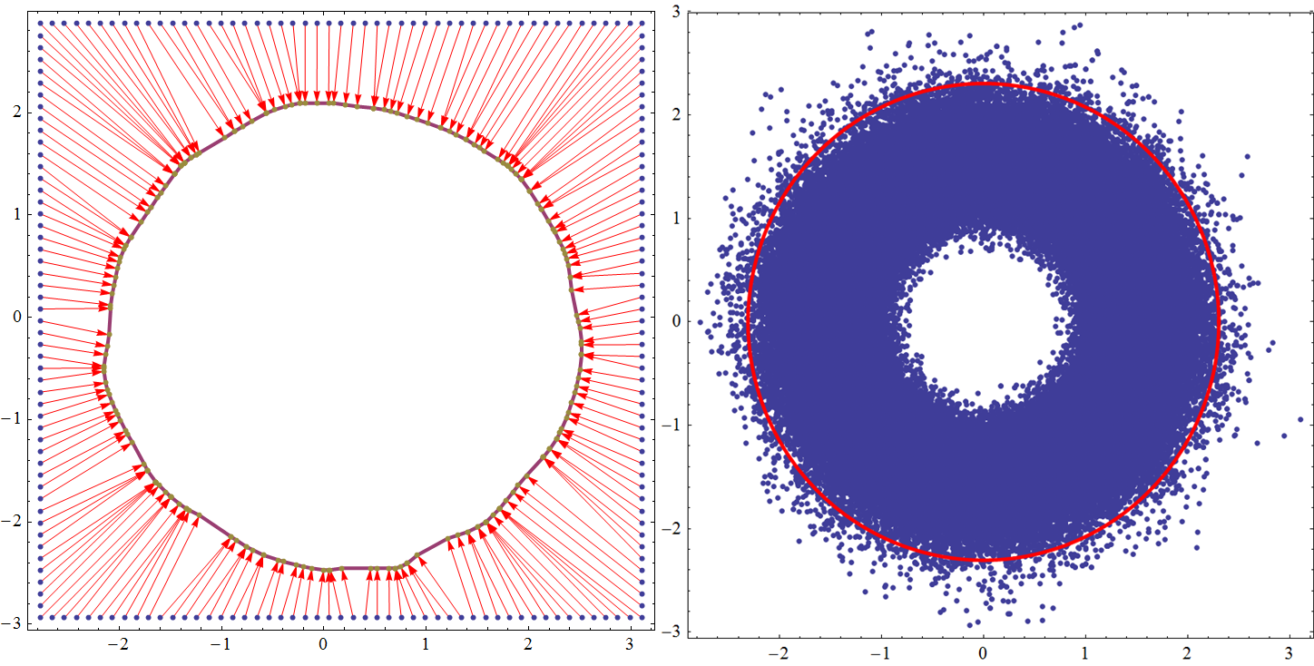
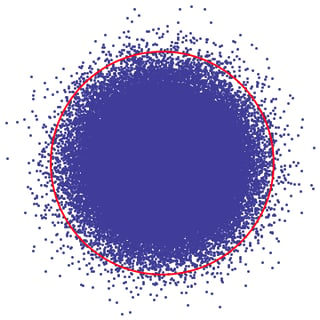
1. In the first pic we can see from the image boundary we detect the points on the outer contour.
2. The second picture draws the circle with a radius that is the median of the norms of the vectors connecting the origin with points forming the target contour.

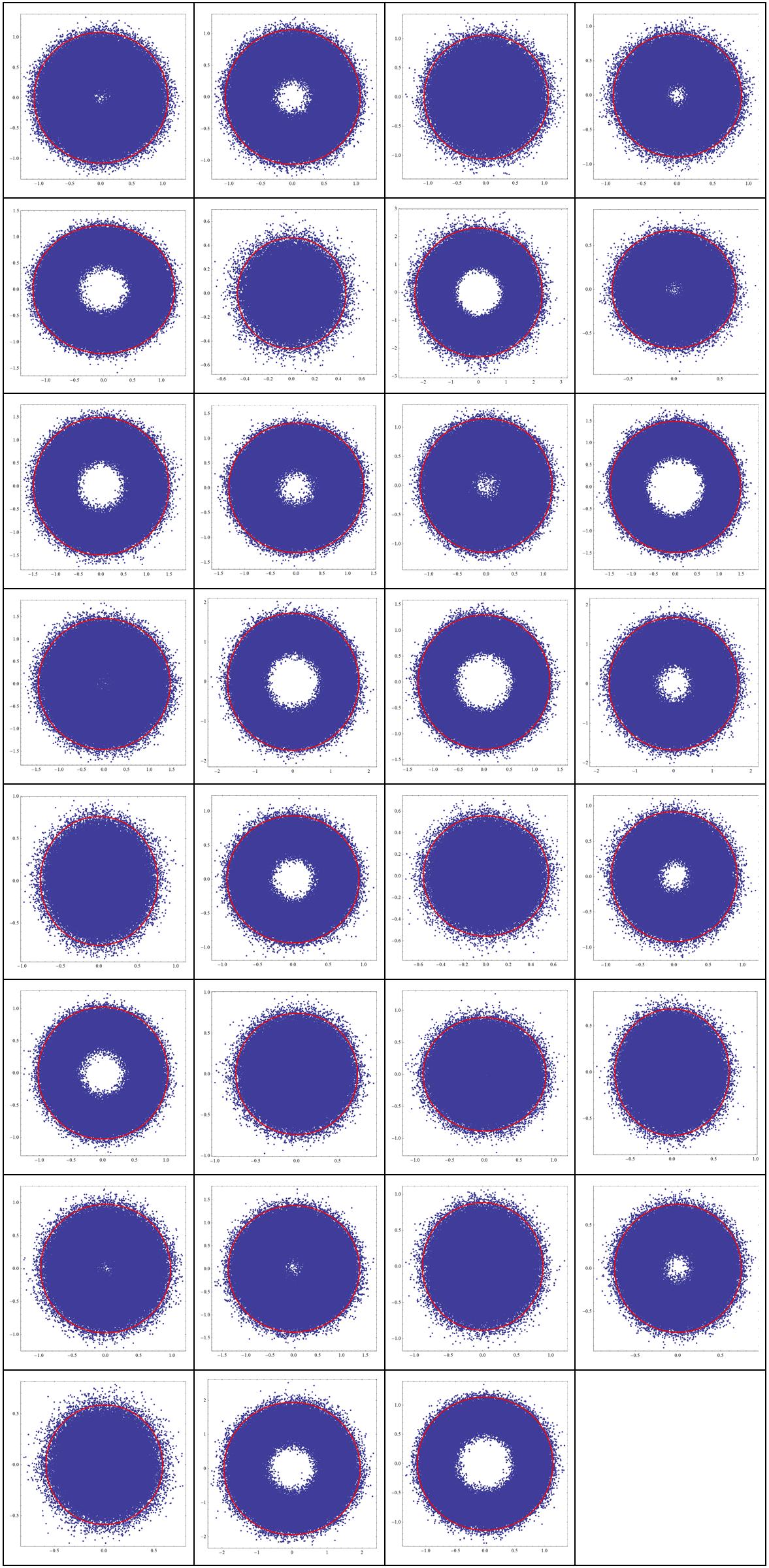
Proof of Robustness:

Questiion:

So far my problem is solved but I am sure one can do this probably more efficiently and elegantly. Any idea for betterment will be helpful. On a sleepless night thought to write a elaborate post....Hope I don't overrun your patience for reading it..

BR

Answer 1

You can use image processing like in the example below to find the enclosing circle. I use FillingTransform to fill in the binarized image, which gives something like the plot on the left. Then using ComponentMeasurements, I obtain the centroid and the radius of a disk that has the same area as the points in the original image. Here's how it looks

data = RandomReal[NormalDistribution[], {100000, 2}]; (* test data *)
p = ListPlot[data, AspectRatio -> 1, Axes -> None];
f = FillingTransform@ColorNegate@Binarize@p // DeleteSmallComponents
{c, r} = 1 /. ComponentMeasurements[f, {"Centroid", "EquivalentDiskRadius"}]    
Show[Rasterize[p], Graphics[{Red, Circle[c, r]}]]

Answer 2

Here is an alternative approach which uses the EllipsoidQuantile function to select points, in this case within two standard deviations. It's not based on image processing, and it could be interesting to see how it compares for your application. In its favour it has a statistical consistency and does not depend on a bespoke program. Some code was reused from belisarius' post on collecting points in an ellipse.

data = Table[RandomVariate[
    BinormalDistribution[{50, 50}, {18, 15}, 0.6]], {2000}];
(* For values within two standard deviations, (approx 95.45% of values) *)
sd = 2;
cl = 2*(CDF[NormalDistribution[0, 1], sd] - 0.5);
Needs["MultivariateStatistics`"];
e = EllipsoidQuantile[data, cl];
ctr = e[[1]];
{r1, r2} = e[[2]];
inc = ArcTan[e[[3, 1, 2]]/e[[3, 1, 1]]]*180/Pi;
Print["Ellipse center = " <> ToString@ctr];
Print["Ellipse radii (r1, r2) = " <> ToString@{r1, r2}];
Print[StringJoin["Ellipse inclination = ", ToString@inc, " degrees"]];

(* Find the foci of the ellipse *)
f = Sqrt[r1^2 - r2^2];
dx = f*Cos[inc Degree];
dy = f*Sin[inc Degree];
f1 = ctr - {dx, dy};
f2 = ctr + {dx, dy};

edge = ctr + r1*e[[3, 1]];
r = EuclideanDistance[edge, f1] + EuclideanDistance[edge, f2];
(* belisarius' code *)
inside[{x_, y_}, {f1_, f2_}] := Sum[
   EuclideanDistance[{x, y}, i], {i, {f1, f2}}];
sd = Select[data, inside[#, {f1, f2}] < r &];

Show[RegionPlot[inside[{x, y}, {f1, f2}] < r, {x, 0, 100}, {y, 0, 100}],
 ListPlot[data],
 Graphics[{Green, Point@sd}],
 Graphics@e,
 Graphics[{Black, Thick, Dashing[0.05],
   Rotate[Circle[ctr, {r1, r2}], inc Degree]}],
 Graphics[{Red, Line[{ctr + r1*e[[3, 1]], ctr, ctr + r2*e[[3, 2]]}]}],
 Graphics[{PointSize[Large], Point[{f1, f2}]}],
 PlotRange -> {{0, 100}, {0, 100}}, AspectRatio -> 1]

Answer 3

you should have a very careful look at MorphologicalComponents, which is part of a really powerful set of functions. You then use ComponentMeasurements to determine the "Bounding disk properties". Appropriate examples are provided by the Help system. Greetings Ernst