Plot of an even/odd function

Question

I have an even function $f(x)$ that I wish to plot on the interval $x \in [-1,1]$. The evaluation of $f(x)$ at a given point takes a bit of time to compute, so I would want to evaluate $f(x)$ only on the interval $x \in [0,1]$ and plot the rest by making use of the evenness of the function. For example, if I do:

myf[x_] := (Pause[0.01]; x^2)
Show[Plot[myf[x], {x, 0, 1}], Plot[myf[x], {x, -1, 0}]],

the second plot is actually a waste.

I could manually make an array of $f(x_i)$ at different points $x_i \in [0,1]$, set $f(-x_i) = f(x_i)$ and then use ListPlot, but I feel that there should be a quicker way to do this. Ideally, something of the sort of using Plot[myf[x], {x, 0, 1}], copy it, make a mirror image of it, stick the two plots together and show the result?

Answer 1

I could manually make an array of f(xi) at different points

You do not need to. Mathematica's Plot does it for you and it is better at sampling at the right places. (adaptive sampling).

How about getting the data points from one half of the plot, and just add minus to each x coordinate?

something like

myf[x_] := x^2
(*read the data from one half only *)
data = Catenate@Cases[Plot[myf[x], {x, 0, 1}], Line[data_] :> data, Infinity];

(*flip the x coordinates*)
data2 = Map[{-First@#, Last@#} &, data];

(*plot both*)
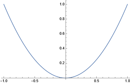
Show[ListLinePlot[data], ListLinePlot[data2], PlotRange -> All]

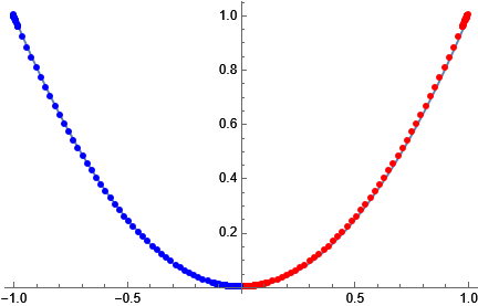
You can see it is the same points used, but one half is flipped

Show[ListLinePlot[data, Mesh -> All, MeshStyle -> Red], 
 ListLinePlot[data2, Mesh -> All, MeshStyle -> Blue], 
 PlotRange -> All]

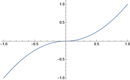
For an odd

data2=Map[{-First@#,-Last@#}&,data];
Show[ListLinePlot[data],ListLinePlot[data2],PlotRange->All]

Answer 2

To complete Nasser's answer, the below shows how to extend the method for a 3D plot, which is inspired by an answer to a different question. Specifically, if $f(x,y)$ is an even function of $x$, then

(* plot f(x,y) for positive x only *)
myplot = Plot3D[x^2 Sin[y], {x, 0, 1}, {y, -\[Pi]/2, \[Pi]/2}];
(* read the data *)
data = FirstCase[myplot, GraphicsComplex[p_, __] :> p, {}, -4];
(* flip x coordinate *)
data2 = Map[{-#[[1]], #[[2]], #[[3]]} &, data];
(* plot both data together *)
Show[ListPlot3D[data], ListPlot3D[data2]]

Answer 3

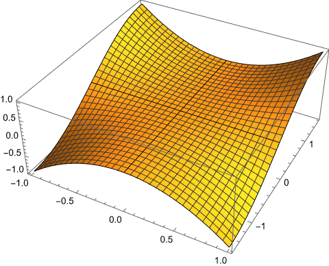
When plotting 3D surfaces with symmetries, it is sometimes convenient to use GeometricTransformation[] with an appropriate choice of ScalingTransform[]. Using the OP's example of a bivariate function with odd and even symmetries:

p1 = Plot3D[x^2 Sin[y], {x, 0, 1}, {y, 0, π/2}];
Graphics3D[GeometricTransformation[First[p1], 
           Table[ScalingTransform[s],
                 {s, {{1, 1, 1}, {-1, 1, 1}, {1, -1, -1}, {-1, -1, -1}}}]], 
           Axes -> Automatic, BoxRatios -> {1, 1, 0.4}]

---

The OP's original parabola example can be treated similarly:

para = Plot[x^2, {x, 0, 1}];
Graphics[GeometricTransformation[First[para],
         Table[{DiagonalMatrix[s], {0, 0}}, {s, {{1, 1}, {-1, 1}}}]], 
         Axes -> Automatic]