(In)Stability of equilibrium points in a vector plot (continued)?

Question

I got a nice answer from Chris to my earlier question(though there are still some points unanswered): (In)Stability of equilibrium points depicted in a vector plot?

Now consider the following system:

$$    
            \begin{align}
            \frac{dS}{dt} &= \nu N -\frac{\beta S I}{N} + \xi R - \nu S\\
            \frac{dE}{dt} &= \frac{\beta S I}{N}- \sigma E -\nu E  \\[2ex]
            \frac{dI}{dt} &= \sigma E -\gamma I -\nu I \\[2ex]
            \frac{dR}{dt} &= \gamma I -\xi R - \nu R
            \end{align}
$$

where $N = S + E + I + R$ is the total population.

If we apply the same technique we have:

r := 1 - s - e - i;
SetModel[{
  Pop[pop] -> {
    Component[s] -> {Equation :> ξ + ν - ξ e - ξ i - β s i  - ξ s - ν s}, 
    Component[e] -> {Equation :>  β s i - σ e - ν e }, 
    Component[i] -> {Equation :> σ e - γ i - ν i }
  },
  Parameters :> {β > 0, γ > 0, ξ > 0, σ > 0, ν > 0}
}]
eq = SolveEcoEq[]

We get:

Which is fine. Now I want to do the following;

β = 0.7; γ = 0.3; σ = 0.3; ξ = 0.4; ν = 0.3;
eq = SolveEcoEq[]
N[EcoEigenvalues[eq[[2]]]]
Show[PlotEcoPhasePlane[{s, 0, 2}, {e, -0.6, 1}], 
 RuleListPlot[eq, PlotMarkers -> EcoStableQ[eq]]]

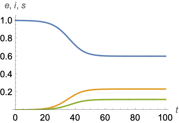
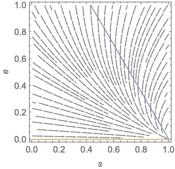
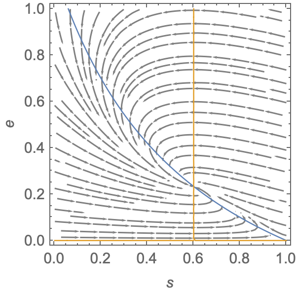
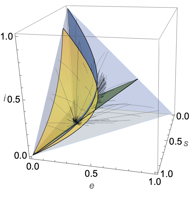
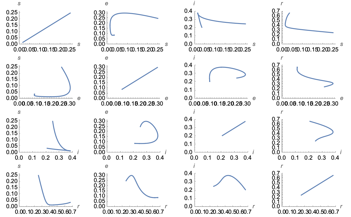
Our system is 3 dimensional so how would I plot phase planes for say $s$ vs $i$ or $s$ vs $e$ etc? What about initial conditions for the phase portraits?

EDIT:

The paper:

https://www.mdpi.com/2227-7390/5/1/7/htm

Hopefully you can recreate the results!

My code for ODE solution:

tmax = 100;
\[Beta] = 4;
\[Sigma] = 1/3;
\[Gamma] = 1/7;
b = (1.9/100)/365;
d = (0.8/100)/365;
\[Alpha] = 1/14;
\[Nu] = 0.8;
\[Rho] = 0.5;
SExPRS = NDSolveValue[{
    S'[t] == \[Alpha] + 
      b (1 - \[Nu]) - \[Alpha]*Ex[t] - \[Alpha]*P[t] - \[Beta]*S[t]*
       P[t] - (b + \[Rho] + \[Alpha])*S[t],
    Ex'[t] == \[Beta]*S[t]*P[t] - (b + \[Sigma])*Ex[t],
    P'[t] == \[Sigma]*Ex[t] - (b + \[Gamma])*P[t],
    S[0] == 0.25,
    Ex[0] == 0.25,
    P[0] == 0.25},
   {S, Ex, P},
   {t, 0, tmax}];
{f1, f2, f3} = SExPRS;

st = Style[#, 15, Black] &;

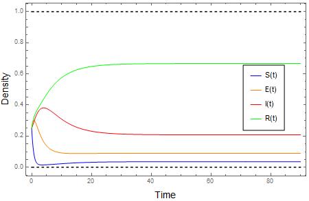
Plot[{f1[t], f2[t], f3[t], 1 - f1[t] - f2[t] - f3[t], 1, 0}, {t, 0, 
  tmax}, PlotStyle -> {Blue, Orange, Red, Green, 
   Directive[Black, Dashed], Directive[Black, Dashed]}, Frame -> True,
  FrameLabel -> st /@ {"Time", "Density"}, 
 PlotLegends -> 
  Placed[LineLegend[{Blue, Orange, Red, Green, Black}, {"S(t)", 
     "E(t)", "I(t)", "R(t)" }, LegendFunction -> Framed], {0.85, 
    0.44}], ImageSize -> 500]

Compared to your eco package:

r := 1 - s - e - i;
SetModel[{Pop[
    pop] -> {Component[
      s] -> {Equation :> \[Xi] + \[Nu] (1 - 
           c) - \[Xi] e - \[Xi] i - \[Beta] s i  - \[Xi] s - \[Nu] s \
- \[Rho] s}, 
    Component[
      e] -> {Equation :>  \[Beta] s i - \[Sigma] e - \[Nu] e }, 
    Component[
      i] -> {Equation :> \[Sigma] e - \[Gamma] i - \[Nu] i }}, 
  Parameters :> {\[Beta] > 0, \[Gamma] > 0, \[Xi] > 0, \[Sigma] > 
     0, \[Nu] > 0, \[Rho] > 0, c > 0}}]
eq = SolveEcoEq[]
    \[Beta] = 4; \[Gamma] = 1/7; \[Sigma] = 1/3; \[Xi] = 
     1/14; c = 0.8; \[Nu] = (1.9/100)/365; \[Rho] = 0.5;
    eq = SolveEcoEq[]
    N[EcoEigenvalues[eq[[2]]]]
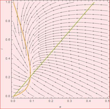
    Show[PlotEcoPhasePlane[{s, 0, 1}, {i, 0, 1}, 
      Fixed -> {e -> \[Sigma]}], 
     RuleListPlot[eq, PlotMarkers -> EcoStableQ[eq]]]
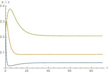
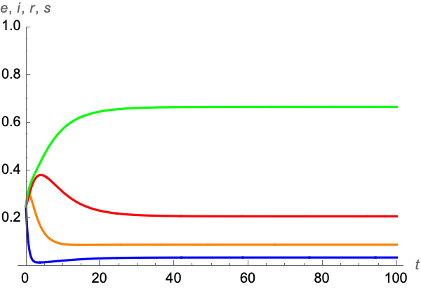
    sol = EcoSim[{s -> 0.25, e -> 0.25, i -> 0.25}, 90];
    PlotDynamics[sol]

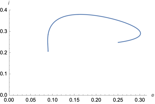
An example of $e$ plotted against $i$:

Answer 1

Nice to see you trying my EcoEvo package. I will increase $\beta$ to get the disease to persist at a stable positive equilibrium.

β = 2;

eq = SolveEcoEq[]
EcoStableQ[eq]
(* {{s -> 1., e -> 0, i -> 0}, {s -> 0.6, e -> 0.233333, i -> 0.116667}} *)
(* {False, True} *)

sol = EcoSim[{s -> 0.999, e -> 0.001, i -> 0}, 100];
PlotDynamics[sol]

PlotEcoPhasePlane takes the option Fixed, which you can use to fix other variables to get a 2D slice. For example,

PlotEcoPhasePlane[{s, 0, 1}, {e, 0, 1}, Fixed -> {i -> 0}]

However, I'm not sure how useful this is, because the fixed variable i actually changes, which you can't see in such a 2D slice of the 3D phase space. One idea would be to assume a quasi-steady state between exposed e and infected i by setting $di/dt=0$, solving for $i$ in terms of $e$, then using that in your 2D phase plane:

PlotEcoPhasePlane[{s, 0, 1}, {e, 0, 1}, Fixed -> {i -> σ e/(γ + ν)}]

Now we can see the stable equilibrium eq[[2]] in a 2D slice.

I haven't built in support for 3D isoclines & streams yet, because I usually find them hard to see. But here's a start at it:

isoclines = ContourPlot3D[
  Evaluate[EcoEqns[] /. ZeroLHS /. var_[t] -> var],
  {s, 0, 1}, {e, 0, 1}, {i, 0, 1},
  ContourStyle -> Opacity[0.8], Mesh -> None, 
  RegionFunction -> Function[{s, e, i}, s + e + i < 1], 
  AxesLabel -> {s, e, i}];

streams = StreamPlot3D[
  Evaluate[EcoEqns[] /. RHS /. var_[t] -> var],
  {s, 0, 1}, {e, 0, 1}, {i, 0, 1}, AxesLabel -> {s, e, i}, 
  RegionFunction -> Function[{s, e, i}, s + e + i < 1], 
  StreamStyle -> {Black, Thin}, StreamColorFunction -> None, 
  StreamPoints -> Fine];

Show[isoclines, streams]

Addition

Given your interests, I suggest including $R$ as a dynamic variable. You can set colors for each variable with Color in SetModel.

SetModel[{
  Pop[pop] -> {
    Component[s] -> {Equation :> ν (1 - c) - β s i - ν s + ξ r - ρ s, Color -> Blue},
    Component[e] -> {Equation :> β s i - σ e - ν e, Color -> Orange},
    Component[i] -> {Equation :> σ e - γ i - ν i, Color -> Red},
    Component[r] -> {Equation :> ν c + γ i - ν r - ξ r + ρ s, Color -> Green}
    }, Parameters :> {β > 0, γ > 0, ξ > 0, σ > 0, ν > 0, ρ > 0, c > 0}}]

To simulate:

β = 4; γ = 1/7; σ = 1/3; ξ = 1/14; c = 0.8; ν = (1.9/100)/365; ρ = 0.5;
sol = EcoSim[{s -> 0.25, e -> 0.25, i -> 0.25, r -> 0.25}, 100];
PlotDynamics[sol, PlotRange -> {0, 1}]

To plot the dynamics of one variable vs another, use RuleListPlot.

RuleListPlot[sol, {e, i}]

Here's a grid of all pairwise combinations:

GraphicsGrid[
  Table[RuleListPlot[sol, {var1, var2}], {var1, {s, e, i, r}}, {var2, {s, e, i, r}}],
  Spacings -> 0]