Stability region of nonlinear ODE system

Question

Sol is the evaluation at $t=100$ of the solution of a nonlinear system of three differential equations with initial values at $a$, $b$, $c$. This is obtained with the function ParametricNDSolveValue.

 sol = ParametricNDSolveValue[
 {x'[t] == -y[t],
  y'[t] == -z[t], 
  z'[t] == -0.915 x[t]+(1-0.915 x[t]^2) y[t]-z[t],
  x[0] == a, y[0] == b, z[0] == c},
 {x[100], y[100], z[100]}, {t, 0, 100}, {a, b, c}
 ]

The point $\{xeq,yeq,zeq\}=\{0,0,0\}$ is one of the stable equilibriums of the alleged system. I would like to obtain the stable region of the this equilibrium so for that I'm trying the following: calculate the distance from a point evaluated with Sol to the equilibrium and then plot all these points. The points I evaluate is the points of the unit cube obtained with a step of 0.1 in each of the coordinates:

Table[EuclideanDistance[sol[a, b, c], {xeq, yeq, zeq}], {a,0, 1,0.1}, {b, 0, 1, 0.1},{c,0,1,0.1}]

This provides me with the distance. The problems are two:

1) I don't know how to obtain back the point $\{a,b,c\}$ (the argument of Sol) for the distances that are less than, say, 0.1 from the equilibrium.

2) I actually have only tried with only one or two variables in a small range, say,

Table[EuclideanDistance[sol[a, b, 0.1], {xeq, yeq, zeq}], {a,0.4, 0.6,0.1}, {b, 0.7, 0.9, 0.1}]

because I usually get the following

General: 1/4.60387*10^307 is too small to represent as a normalized machine number; precision may be lost.

which makes the evaluation last forever not showing any outcome.

How can I overcome these issues?

Answer 1

Here's a way rather in line with the OP's approach:

(* returns the squared distance to the origin *)
sol = ParametricNDSolveValue[{x'[t] == -y[t], y'[t] == -z[t], 
    z'[t] == -0.915 x[t] + (1 - 0.915 x[t]^2) y[t] - z[t], x[0] == a, 
    y[0] == b, z[0] == c,
    WhenEvent[
     x[t]^2 + y[t]^2 + z[t]^2 < Min[(a^2 + b^2 + c^2)/100, 10^-6], 
     "StopIntegration"]},
   Indexed[x["ValuesOnGrid"], -1]^2 +   (* This is the same idea as KraZug's *)
    Indexed[y["ValuesOnGrid"], -1]^2 +  (* use of the last value, but with a *)
    Indexed[z["ValuesOnGrid"], -1]^2,   (* different code *)
   {t, 0, 100}, {a, b, c}];

stab = RegionPlot3D[
    Quiet@sol[a, b, c] < 1  (* a smaller threshold is not really necessary *)
    {a, -2, 2}, {b, -2, 2}, {c, -2, 2}, 
    Mesh -> None]; // AbsoluteTiming
(*  {29.8274, Null}  <-- Takes a while! *)

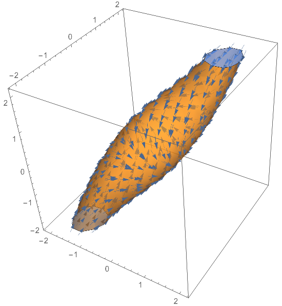
We'll show the region with the flow indicated on the surface, which should be tangent to it (to the gold part, not the blue part). We can see that the stability region extends further out the top and bottom:

(* lazy way to get the vector field *)
{state} = NDSolve`ProcessEquations[{x'[t] == -y[t], y'[t] == -z[t], 
    z'[t] == -0.915 x[t] + (1 - 0.915 x[t]^2) y[t] - z[t],
    x[0] == 1, y[0] == 2, z[0] == 3}, (* random IC, not used *)
    {x, y, z}, {t, 0, 100}
   ];
nf = state@"NumericalFunction";

Show[Cases[stab, 
  GraphicsComplex[p_, ___] :> 
   VectorPlot3D[nf[0, {a, b, c}], {a, -2, 2}, {b, -2, 2}, {c, -2, 2}, 
    VectorPoints -> p, VectorScale -> {0.045, Automatic, None}], 
  Infinity],
 stab /. RGBColor[r_, g_, b_] :> RGBColor[r, g, b, 0.6] (* opacity was an afterthought *)
 ]

If you want to use a greater number of PlotPoints in RegionPlot, you can downsample the points for VectorPlot with something like the following:

VectorPoints -> Union[p, SameTest -> (EuclideanDistance[##] < 0.2 &)]

Answer 2

So the issue is that at some parameter the solution diverges, which then gives vectors that are too large to use EuclideanDistance on. So we need to catch that, for instance in this way:

sol = ParametricNDSolveValue[{x'[t] == -y[t], y'[t] == -z[t], 
   z'[t] == -0.915 x[t] + (1 - 0.915 x[t]^2) y[t] - z[t], x[0] == a, 
   y[0] == b, z[0] == c}, {x, y, z}, {t, 0, 10000}, {a, b, c}]

tab = Flatten[Table[cursol = sol[a, b, c];
    endpt = cursol[[1, 1, 1, 2]];
    {a, b, c, EuclideanDistance[Through[cursol[endpt]], {0, 0, 0}]}, {a, 0, 
     1, 0.1}, {b, 0, 1, 0.1}, {c, 0, 1, 0.1}], 2];

Here sol now returns the whole interpolation function, and cursol[[1, 1, 1, 2]] digs into the interpolation functions to return the endpoint of the integration. The table returns a list {x,y,z,f}, which we can split based on the values of f:

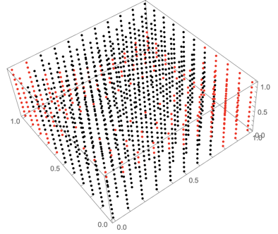
ListPointPlot3D[{Select[tab, #[[4]] < 0.01 &][[All, 1 ;; 3]], 
  Select[tab, #[[4]] >= 0.01 &][[All, 1 ;; 3]]}, 
 PlotStyle -> {Black, Red}]