Local optimization of parameters in a Coupled Non-Linear System

Question

I have a system of differential equations :

$\frac{dX}{dt} = (0.8+0.4c_{1})X-(0.007+0.006c_{2})XY$ and

$\frac{dY}{dt} = (0.048+0.004c_{3})XY-(0.4+0.2c_{4})Y$

where $0\le c_{i}\le1$.

Varying $c_{i}$ gives me an envelope of solutions for both $X(t)$ and $Y(t)$. My goal is to find the combination of $c_{i}$ which gives the upper and lower limits of my solution.

Taking $c_{i}$ as discrete points between 0 and 1 with step size 0.1, I used the following code to obtain a solution, and managed to plot it.

sol = ParametricNDSolve[{x'[t] == (0.8 + 0.4 c1) x[t] - (0.007 + 0.006 c2) x[t] y[t],y'[t] == (0.0048 + 0.0004 c3) x[t] y[t] - (0.4 + 0.2 c4) y[t], x[0] == 200, y[0] == 80}, {x, y}, {t, 0, 50}, {c1, c2, c3, c4}]
xt = Flatten[Evaluate[Table[x[c1, c2, c3, c4][t] /. sol, {c1, 0, 1, 0.1}, {c2, 0, 1,0.1}, {c3, 0, 1, 0.1}, {c4, 0, 1, 0.1}]]];
mat = Table[Table[Evaluate[xt[[a]]], {t, 0, 25, 0.01}], {a,Range[Length[xt]]}];
l = Min /@ Transpose[mat];
m = Max /@ Transpose[mat];
ind = Range[0, 25, 0.01];
lupd = Transpose[{ind, l}];
mupd = Transpose[{ind, m}];
ListLinePlot[{lupd, mupd},GridLines -> Automatic, ImageSize -> {600, 300}]

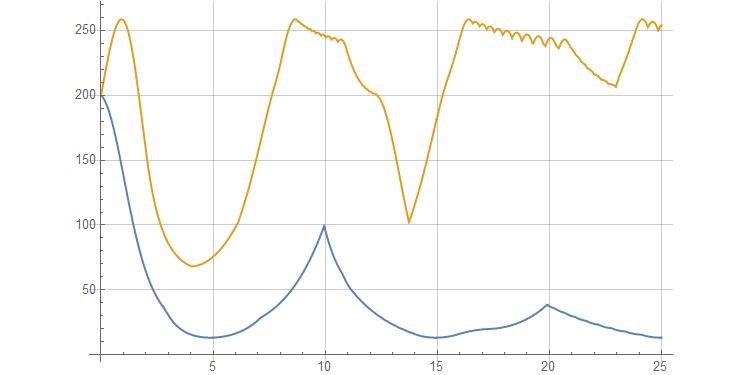
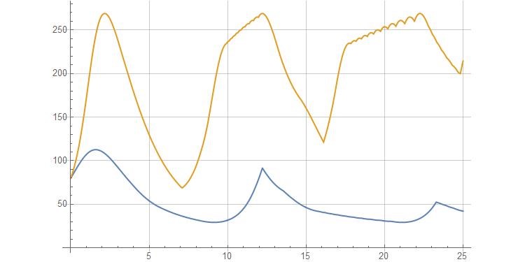
The plot for $X(t)$ came as The plot for $Y(t)$ came as Edit 3

It is not possible to calculate the equation of the upper curve of the envelope obtained by varying $c_{i}$s. Hence, I reworked my question.

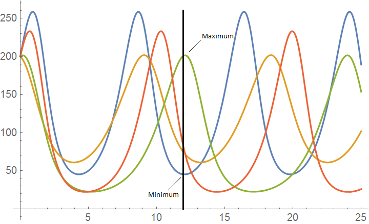
Consider the following code fragment

Plot[Evaluate@({x[1, 0, 0, 1][t], x[0, 1, 1, 1][t], x[0, 0, 0, 0][t], 
     x[0.8, 0, 0, 0.2][t]} /. sol), {t, 0, 25}]

This gives 4 different trajectories for $X(t)$.

Consider the line $t=12$. As it cuts the enevelope, we get a minimum point and a maximum point.

I would like the combination of $c_{i}$ that give this maximum and minimum points for $t=1,2,3,...,25$.

In my solution I used Max and Min to extract these maximum and minimum points and then plotted them. I could not get the combination of $c_{i}$ for each of these points.

Answer 1

As I pointed out in the comments, the $c_i$ do not retain the frequency of the solutions constant so the solutions cross each other and there isn't one collection of $ c_i $ that satisfies the "maximum envelope" criterion. For different integer times it's an easy application of NMaximize:

Table[NMaximize[{x[c1, c2, c3, c4][t] /. sol, 0 <= c1 <= 1, 0 <= c2 <= 1, 0 <= c3 <= 1, 0 <= c4 <= 1}, {c1, c2, c3, c4}], {t, 1, 25}]

which produces a solution (but doesn't always converge properly so maybe some playing around with the parameters of NMaximize is necessary here):

{{311.231, {c1 -> 1., c2 -> 0., c3 -> 0., 
   c4 -> 1.}}, {195.645, {c1 -> 0.851284, c2 -> 0., c3 -> 0., 
   c4 -> 1.}}, {101.746, {c1 -> 0., c2 -> 0., c3 -> 0., 
   c4 -> 1.}}, {72.4078, {c1 -> 0.554206, c2 -> 1., c3 -> 0., 
   c4 -> 1.}}, {86.7196, {c1 -> 0.516399, c2 -> 1., c3 -> 0., 
   c4 -> 1.}}, {119.434, {c1 -> 0.783024, c2 -> 1., c3 -> 0., 
   c4 -> 1.}}, {174.87, {c1 -> 1., c2 -> 1., c3 -> 0., 
   c4 -> 1.}}, {225.381, {c1 -> 1., c2 -> 0.393763, c3 -> 0., 
   c4 -> 1.}}, {312.48, {c1 -> 1., c2 -> 0., c3 -> 0., 
   c4 -> 1.}}, {298.507, {c1 -> 1., c2 -> 0., c3 -> 0., 
   c4 -> 0.483703}}, {289.22, {c1 -> 1., c2 -> 0., c3 -> 0., 
   c4 -> 0.0869823}}, {242.738, {c1 -> 0.536497, c2 -> 0., c3 -> 0., 
   c4 -> 0.}}, {206.276, {c1 -> 0., c2 -> 4.11611*10^-9, 
   c3 -> 8.75751*10^-6, c4 -> 0.}}, {143.553, {c1 -> 1., c2 -> 1., 
   c3 -> 0., c4 -> 1.}}, {196.936, {c1 -> 1., c2 -> 1., c3 -> 0., 
   c4 -> 1.}}, {245.969, {c1 -> 1., c2 -> 0.331846, c3 -> 0., 
   c4 -> 1.}}, {313.172, {c1 -> 1., c2 -> 0., c3 -> 0., 
   c4 -> 1.}}, {304.824, {c1 -> 1., c2 -> 0., c3 -> 0., 
   c4 -> 0.715149}}, {298.267, {c1 -> 1., c2 -> 0., c3 -> 0., 
   c4 -> 0.4678}}, {293.266, {c1 -> 1., c2 -> 0.0000225295, 
   c3 -> 2.52908*10^-7, c4 -> 0.262797}}, {281.43, {c1 -> 0.99607, 
   c2 -> 0.00393228, c3 -> 0.739327, 
   c4 -> 0.108152}}, {270.711, {c1 -> 0.939643, c2 -> 0.000403377, 
   c3 -> 0.999011, c4 -> 0.000087475}}, {211.763, {c1 -> 1., 
   c2 -> 0.757642, c3 -> 0., c4 -> 1.}}, {261.286, {c1 -> 1., 
   c2 -> 0.265911, c3 -> 0., c4 -> 1.}}, {313.282, {c1 -> 1., 
   c2 -> 0., c3 -> 0., c4 -> 1.}}}