Nonlinear Model Fitting to Numerical Data with automatic elimination

Question

I have an experimental data set {f,x,y,z} as

{{300., 2., 4., 6.}, {500., 0., 4., 25.}, {6600., 1., 15., 9.}, {100., 5., 0., 2.}, {1100., 10., 8., 1.}, {1300., 7., 8., 18.}, {300., 23., 5., 0.}, {400., 1., 5., 3.}, {900., 3., 7., 9.}, {800., 4., 7., 2.}, {400., 4., 4., 11.}, {3300., 24., 12., 0.}, {600., 2., 6., 8.}, {300., 2., 4., 6.}, {600., 22., 6., 7.}, {17900., 3., 21., 44.}}

I need to find the best fitted parameters for the function:

f=a*(x*b)^0.3 + c*(y*d)^3 + e*(z*h)^g

where a, b, c, d, e, h, g is the fitted parameters. The problem is how to drop a certain data line with a higher deviation than a certain value e.g greater than 10% and then restart the finding parameters to have the best fitted parameters. The another problem is how to guess the initials (starting points) for the parameters. Could you please advise how to solve the problem? Thank you.

Answer 1

I'm not a fan of automatically tossing data (although the RANSAC algorithm mentioned by @Roman is great for finding potential outliers - just as long as one doesn't toss data without thinking especially if you have only 16 data points and are fitting 5 parameters: $a$, $c$, $e$, $g$, and the error variance).

But in this case your model doesn't seem to produce any outliers and ends up with a near perfect fit.

To get NonlinearModelFit to get you parameter estimates (but no estimates of associated standard errors) one needs to use Method = "NMinimize":

data = {{300, 2, 4, 6}, {500, 0, 4, 25}, {6600, 1, 15, 9}, {100, 5, 0, 2}, {1100, 10, 8, 1}, 
  {1300, 7, 8, 18}, {300, 23, 5, 0}, {400, 1, 5, 3}, {900, 3, 7, 9}, {800, 4, 7, 2}, 
  {400, 4, 4, 11}, {3300, 24, 12, 0}, {600, 2, 6, 8}, {300, 2, 4, 6}, {600, 22, 6, 7}, 
  {17900, 3, 21, 44}};
(* Rearrange data to form needed by NonlinearModelFit *)
data[[All, {2, 3, 4, 1}]] = data;

nlm = NonlinearModelFit[data, {a x^(3/10) + c y^3 + e z^g, a > 0 && c > 0 && e > 0 && g > 0}, 
  {a, c, e, g}, {x, y, z}, Method -> "NMinimize", MaxIterations -> 5000];
nlm["BestFitParameters"]
(* {a -> 18.0549, c -> 1.88037, e -> 71.9428, g -> 0.496803} *)

I think that Method -> "NMinimize" is needed because without that the part of the model with e z^g chokes on the values of z that are zero. This also probably causes the inability to produce standard errors of the parameters. (Maybe there's a simple way to get around that.)

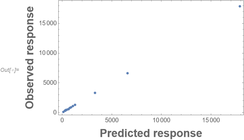
A plot of the predicted value vs. the observed value doesn't show (to me) any abnormalities:

ListPlot[Transpose[{nlm["PredictedResponse"], data[[All, 4]]}], Frame -> True, 
  FrameLabel -> (Style[#, Bold, 18] &) /@ {"Predicted response", "Observed response"},
  PlotRange -> All]

The adjusted $R^2$ value is

nlm["AdjustedRSquared"]
(* 0.999971 *)

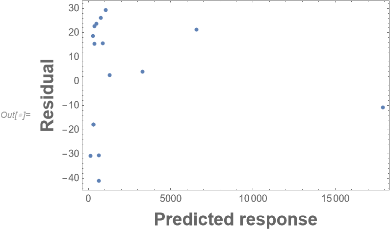
A plot of the residuals vs the predicted value also shows no abnormalities:

ListPlot[Transpose[{nlm["PredictedResponse"], nlm["FitResiduals"]}], Frame -> True, 
  FrameLabel -> (Style[#, Bold, 18] &) /@ {"Predicted response", "Residual"},
  PlotRange -> All]

If what you presented was just an example dataset and still want to know how to use something like the RANSAC algorithm, then having a dataset with at least one obvious outlier would be better.

If, however, this is the dataset of interest and standard errors are needed for the parameters, then that can be added.