Nonlinear model fit with Numerical integration

Question

I'm having trouble writing a Nonlinear Model fit where the model is a numerical integral evaluated with NIntegrate. I have read other questions and answers about more or less the same problem, but for some reason I cannot make sense of this. Here goes:

I define a function containing the integral:

    LumDist[zmax_?NumericQ, Om_?NumericQ, Ol_?NumericQ, Ot_?NumericQ, 
  n_?NumericQ] := NIntegrate[1/\[Sqrt](Om*(1 + x)^3 + Ol + Ot*(1 + x)^n), {x, 0, zmax}]

and from there define the model:

DistMod[zmax_?NumericQ, Om_?NumericQ, Ol_?NumericQ, Ot_?NumericQ, 
  n_?NumericQ, mu0_?NumericQ] := 
 5*Log10[LumDist[zmax, Om, Ol, Ot, n]] + mu0

From here I write a NonlinearModelFit for this model (data) is an (x,y) List:

lmvar = NonlinearModelFit[
  data, {DistMod[z, 0.28, 0.71, Ot, 10^(-3), mu0], 
   1 < Ot >= 0}, {{Ot, 0.08}, {mu0, 23.89}}, x, Weights -> 1/errors^2,
   VarianceEstimatorFunction -> (1 &), Method -> "NMinimize"]

But this does not work, and I get lots of errors such as:

NIntegrate::nlim: x = z is not a valid limit of integration. >>

and

NIntegrate::itraw: Raw object 0.01012` cannot be used as an iterator. >>

Here is a sample of the data and errors:

data = {{0.015, 34.1114},{0.0277, 35.705},{0.048948, 36.7316},{0.0651, 37.3067},{0.100915, 38.4567},{0.159, 39.4164},{0.248508, 40.2722},{0.455, 42.3239},{0.655, 42.3151},{0.75, 43.243},{0.84, 43.5143},{0.961, 44.2642},{1.188, 44.6076},{1.34, 45.0675},{1.414, 44.8038}}

errors={0.215239,0.118114,0.175773,0.242628,0.121087,0.21481,0.152213,0.306006,0.188809,0.198402,0.471047,0.1534, 0.421,0.213,0.1345}

Can anyone tell me what I am doing wrong here?

Moreover, I can even write another simpler model (it's completely wrong, but I want to try to isolate the problem):

testfunc[a_?NumericQ, x_?NumericQ] := NIntegrate[a*t, {t, 1, x}];

Which I can try to fit using:

NonlinearModelFit[data, {testfunc[b], b > 0.}, b, x, 
 Method -> "NMinimize"]

but this also throws lots of errors, such as:

NonlinearModelFit::nrnum: The function value 1/2 ((-26.877+testfunc[0.0914636])^2+(-26.2011+testfunc[0.0914636])^2+(-26.1609+testfunc[0.0914636])^2+(-26.0592+testfunc[0.0914636])^2+(-26.0071+testfunc[0.0914636])^2+(-25.9072+testfunc[0.0914636])^2+(-25.7394+testfunc[0.0914636])^2+(-25.6034+testfunc[0.0914636])^2+<<35>>+(-24.5574+testfunc[0.0914636])^2+(-24.548+testfunc[0.0914636])^2+(-24.5443+testfunc[0.0914636])^2+(-24.5128+testfunc[0.0914636])^2+(-24.4717+testfunc[0.0914636])^2+(-24.4442+testfunc[0.0914636])^2+(-24.4217+testfunc[0.0914636])^2+<<996>>) is not a real number at {b} = {0.0914636}. >>

Answer 1

The fundamental problem with your simplified example is that you don't explicitly incorporate x in NonlinearModelFit. A solution, albeit a completely incorrect one, can be found with a slight modification to NonlinearModelFit:

testfunc[a_?NumericQ, x_?NumericQ] := NIntegrate[a*t, {t, 1, x}];
NonlinearModelFit[data, {testfunc[b,x], b > 0.}, b, x, Method -> "NMinimize"]

To really test what is going on here, a slightly more flexible model could be introduced. Changing testfunc just a bit:

testfunc[a_?NumericQ, b_?NumericQ, x_?NumericQ] := NIntegrate[a*t^b, {t, 0, x}];

Now, NonlinearModelFit can be used to find a reasonable fit:

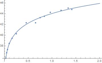
nlm = NonlinearModelFit[data, {testfunc[a, b, x], a > 0, b < 0}, {a, b}, x]
(*FittedModel[testfunc[2.65151,-0.939799,x]]*)

nlm["ParameterTable"]
(*  
Estimate    Standard Error  t-Statistic P-Value
a   2.65151 0.0537729   49.3094 3.59017*10^-16
b   -0.939799   0.00114251  -822.574    4.78556*10^-32
*)

Showing the solution:

There is a similar error in the definition of the actual function of interest. You should be able to find a fit with:

LumDist[zmax_?NumericQ,Om_?NumericQ,Ol_?NumericQ,Ot_?NumericQ,n_?NumericQ]:=NIntegrate[1/\[Sqrt](Om*(1+x)^3+Ol+Ot*(1+x)^n),{x,0,zmax}]
DistMod[zmax_?NumericQ,Om_?NumericQ,Ol_?NumericQ,Ot_?NumericQ,n_?NumericQ,mu0_?NumericQ]:=5*Log10[LumDist[zmax,Om,Ol,Ot,n]]+mu0

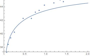
lmvar=NonlinearModelFit[data,{DistMod[z,0.28,0.71,Ot,10^(-3),mu0],0<= Ot<1},{{Ot,0.08},{mu0,23.89}},z,Weights->1/errors^2,VarianceEstimatorFunction->(1&)]

(*FittedModel[DistMod[z,0.28,0.71,0.999999,1/1000,44.5454]]*)

lmvar["ParameterTable"]
(*
    Estimate    Standard Error  t-Statistic P-Value
Ot  0.999999    0.727728    1.37414 0.192627
mu0 44.5454 0.3562  125.057 2.05428*10^-21
*)

Show[Plot[lmvar[x], {x, 0, 2}], ListPlot[data]]

Note, the problem with the original call to NonlinearModelFit did not include the dependent variable (in this case z). You might be able to find a better fit playing around with the options of NonlinearModelFit.

Answer 2

Update

One of the problems is that the model is over-parameterized by 2 or more parameters. Below are some algebraic steps that shows at least two of the parameters can be replaced by a single parameter. (That at least two additional parameters can be replaced by a single parameter is not shown but the evidence is in examining the parameter CorrelationMatrix from NonlinearModelFit.) This suggests that either just taking the logs of the response and predictor variable and fitting a straight line is what should be done or rethinking of the original model is necessary.

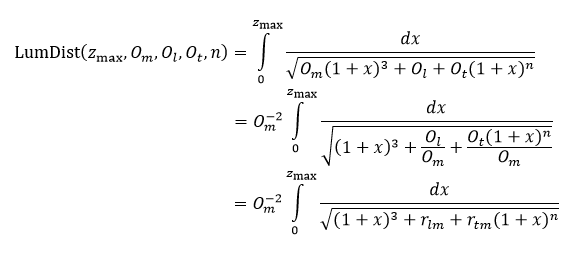
Here is the definition of LumDist where we extract Om:

The final model (DistMod) can therefore be written as follows:

We see that we can only at best estimate $-10 \log_{10} O_m+\mu_0$ and not $O_m$ and $\mu_0$ separately.

End of update

There are (still) a few typos in the original question. If x is changed to z in the NonlinearModelFit statement, the restriction 1 < Ot >= 0 is changed to 0 <= Ot < 1 (or as written it might even be equivalent to Ot > 1 - can't really tell), and VarianceFunctionEstimation is removed, the model converges:

lmvar = NonlinearModelFit[data, {DistMod[z, 0.28, 0.71, Ot, 10^(-3), mu0], 0 <= Ot < 1},
   {{Ot, 0.08}, {mu0, 23.89}}, z, Weights -> 1/errors^2];
lmvar["ParameterTable"]

$$\begin{array}{l|llll} \text{} & \text{Estimate} & \text{Standard Error} & \text{t-Statistic} & \text{P-Value} \\ \hline \text{Ot} & 0.999999 & 2.42865 & 0.411751 & 0.68723 \\ \text{mu0} & 44.5454 & 1.18875 & 37.4725 & \text{1.2436775876447106$\grave{ }$*${}^{\wedge}$-14} \\ \end{array}$$

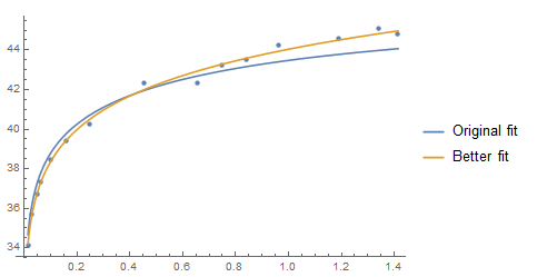
It appears that the use of the parameter Ot is not very useful as the fit is poor and the estimate is at the boundary.

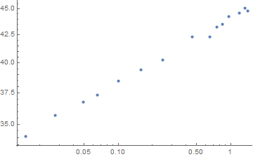
A much better fit can be found by noting that a log-log plot appears to be a simple straight line

ListLogLogPlot[data]

Fitting such a model we have

lmvar2 = NonlinearModelFit[Log[data], a + b logx, {a, b}, logx];
lmvar2["ParameterTable"]

$$\begin{array}{l|llll} \text{} & \text{Estimate} & \text{Standard Error} & \text{t-Statistic} & \text{P-Value} \\ \hline a & 3.7851 & 0.00207508 & 1824.07 & \text{1.526517371336953$\grave{ }$*${}^{\wedge}$-36} \\ b & 0.0601371 & 0.00104813 & 57.3755 & \text{5.051558118117479$\grave{ }$*${}^{\wedge}$-17} \\ \end{array}$$

Show[ListPlot[data], 
 Plot[{lmvar[z], Exp[lmvar2[Log[z]]]}, {z, Min[data[[All, 1]]], 
   Max[data[[All, 1]]]},
  PlotLegends -> {"Original fit", "Better fit"}]]

Assuming that the full dataset has a similar look and feel, this new approach not only provides a better fit but is much faster.

(I note that despite Wolfram producing an example as to how to fit curves when there is measurement error, that example assumes (generally inappropriately) that there is only measurement error and assumes the more typical lack-of-fit error is zero. So given that the measurement errors in this example (which I assume are standard deviations) are pretty similar among themselves, I'd even drop the use of Weights.)