4
$\begingroup$

I have a list of points $(x, y)$, and I expect them to be related as $$y = a(b-x)^c,$$ where $a$, $b$, and $c$ are unknown constants. I also know the approximate values of constants, which can be used as initial guess.

How can I fit the curve to my data?

I tried using NonlinearModelFit, but it returns errors. Here, the actual values (which I am trying to estimate) are $a = 1, b = 1, c = 0.5$.

data = N[Table[{n/50, Sqrt[1 - n/50] + RandomReal[]/10}, {n, 1, 49}]]
(* {{0.02, 0.989949}, {0.04, 0.979796}, {0.06, 0.969536}, {0.08, 
  0.959166}, {0.1, 0.948683}, {0.12, 0.938083}, {0.14, 
  0.927362}, {0.16, 0.916515}, {0.18, 0.905539}, {0.2, 
  0.894427}, {0.22, 0.883176}, {0.24, 0.87178}, {0.26, 
  0.860233}, {0.28, 0.848528}, {0.3, 0.83666}, {0.32, 
  0.824621}, {0.34, 0.812404}, {0.36, 0.8}, {0.38, 0.787401}, {0.4, 
  0.774597}, {0.42, 0.761577}, {0.44, 0.748331}, {0.46, 
  0.734847}, {0.48, 0.72111}, {0.5, 0.707107}, {0.52, 0.69282}, {0.54,
   0.678233}, {0.56, 0.663325}, {0.58, 0.648074}, {0.6, 
  0.632456}, {0.62, 0.616441}, {0.64, 0.6}, {0.66, 0.583095}, {0.68, 
  0.565685}, {0.7, 0.547723}, {0.72, 0.52915}, {0.74, 
  0.509902}, {0.76, 0.489898}, {0.78, 0.469042}, {0.8, 
  0.447214}, {0.82, 0.424264}, {0.84, 0.4}, {0.86, 0.374166}, {0.88, 
  0.34641}, {0.9, 0.316228}, {0.92, 0.282843}, {0.94, 
  0.244949}, {0.96, 0.2}, {0.98, 0.141421}} *)

fit = NonlinearModelFit[data, {a (b - q)^c}, {{a, 0.8}, {b, 0.9}, {c, 0.6}}, q, 
  Method -> NMinimize]

NonlinearModelFit::nrnum: The function value 1.50013 -0.120551 I is not a real number at {a,b,c} = {0.8,0.9,0.6}.

NMinimize::nnum: The function value Experimental`NumericalFunction[{Hold[Block[{q={0.02,0.04,0.06,0.08,0.1,0.12,0.14,0.16,0.18,0.2,<<39>>},Optimization`FindFit`y$1610={0.989949,0.979796,0.969536,0.959166,0.948683,0.938083,0.927362,0.916515,0.905539,0.894427,<<39>>}},1/2 (Times[<<2>>]-Optimization`FindFit`y\$1610).(Times[<<2>>]-Optimization`FindFit`y\$1610)]],Block},{0,{{{},1,0,Hold[0.8],0,0},{{},1,1,Hold[0.9],0,0},{{},1,2,Hold[0.6],0,0}}},<<3>>,{None,None,None}][{0.8,0.9,0.6}] is not a number at {a,b,c} = {0.8,0.9,0.6}.

$\endgroup$
2
  • $\begingroup$ What error structure are you considering? $\endgroup$
    – JimB
    Commented Aug 11, 2023 at 21:21
  • $\begingroup$ Some random numbers. I have updated In[1] with my error structure. $\endgroup$ Commented Aug 11, 2023 at 21:44

6 Answers 6

6
$\begingroup$

Method-1

  • Remove the restriction of a and b.Also remove the Method -> "NMinimize.
data = N[Table[{n/50, Sqrt[1 - n/50] + RandomReal[]/10}, {n, 1, 49}]];
nlm = NonlinearModelFit[data, {a (b - x)^c}, {a, b, {c, .6}}, x]
Plot[nlm[x], {x, 0, 1}, Epilog -> {Red, Point[data]}, 
 AspectRatio -> Automatic]

enter image description here

Method-2

  • If we want the c near .5, the initial value of c may set to be (c - .6) etc.
data = N[Table[{n/50, Sqrt[1 - n/50] + RandomReal[]/10}, {n, 1, 49}]];
nlm = NonlinearModelFit[data, {a (b - x)^(c - .6)}, {a, b, c}, x]

Plot[nlm[x], {x, 0, 1}, Epilog -> {Red, Point[data]}, 
 AspectRatio -> Automatic]

enter image description here

Method-3

  • Or add a perturbation of the exponent.
Clear["Global`*"];
data = N[
   Table[{n/50, Sqrt[1 - n/50] + RandomReal[]/10}, {n, 1, 49}]];
nlm = NonlinearModelFit[data, {a (b - x)^(c + d)}, {a, b, c, d}, x]
Plot[nlm[x], {x, 0, 1}, Epilog -> {Red, Point[data]}, 
 AspectRatio -> Automatic]

enter image description here

$\endgroup$
1
  • $\begingroup$ A question about the syntax: Does NonlinearModelFit[data, {a (b - x)^(c - .6)}, {a, b, c}, x] set the initial value of c to be 0.6? If so, how is that different from NonlinearModelFit[data, {a (b - x)^c}, {a, b, {c,0.6}}, x]? $\endgroup$ Commented Aug 12, 2023 at 20:05
5
$\begingroup$

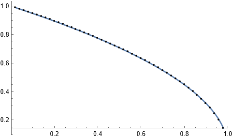
If appropriate to better understand the functional form near x=1 just fit that portion of the data.

fit = NonlinearModelFit[data[[30 ;;]], {a (b - x)^c }, {a, b, c}, x];
Plot[fit[x], {x, 0.02, 0.98}, Epilog -> Point[data]]

However the fit is still not the best.

enter image description here

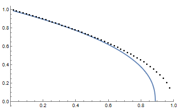
Altering the parameterization greatly improves the fit.

fit = NonlinearModelFit[data[[30 ;;]], {a (b - x)^c - d}, {a, b, c, d}, x];
Plot[fit[x], {x, 0.02, 0.98}, Epilog -> Point[data]]

enter image description here

$\endgroup$
1
  • 2
    $\begingroup$ Any intuitive idea why subtracting d improves it so much? In the original table data, the value of d is zero. $\endgroup$ Commented Aug 11, 2023 at 22:45
4
$\begingroup$

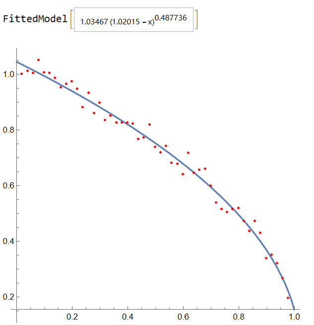
For some values of a,b,c y may be complex. MMA gives you a warning but gets nevertheless a fit:

MMA version 13.3 Windows 10

fit = NonlinearModelFit[data, {a (b - x)^c}, {a, b, c}, x];
Plot[fit[x], {x, 0.02, 0.98}, Epilog -> Point[data]]

enter image description here

$\endgroup$
2
  • 3
    $\begingroup$ Is there any way to obtain a better fit? The fit does not match the points very well near x=1. I am trying to numerically obtain some critical exponents, and the behavior near the point where y becomes 0 is most crucial for me. If you want, I can ask a new question. $\endgroup$ Commented Aug 11, 2023 at 20:30
  • $\begingroup$ The formula a (b - x)^c together with a least square fit does not fit the data very well. What you can try is a weighted fit and give the values near 1 less weight. With this the errors in the fit will be larger near 1 and give a better fit after taking the exponential. $\endgroup$ Commented Aug 12, 2023 at 6:57
4
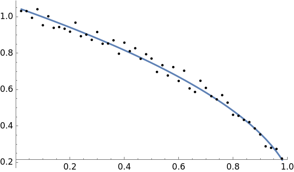
$\begingroup$

This gives a result similar to some of the others posted. The idea is to linearize the objective function by taking logs. This means sweeping b and the x values inside a log together so we create a function for that purpose and use it in the defining objective.

I had to use NMinimize because FindMinimum, at least with default settings, was unwilling to move from the initial values.

logx[b_, vals_] := Log[b - vals]

bestFit[data_] := Module[
  {xvals, yvals, obj, ly, y},
  {xvals, yvals} = Transpose[data];
  obj[a_Real, b_Real, c_Real] := 
   Module[{ovec = 
      Log[yvals] - (Log[a] + c*logx[b, xvals]) /. 
       Indeterminate :> Nothing, res},
    Abs[ovec . ovec]];
  NMinimize[obj[a, b, c], {{a, .7, .9}, {b, .8, .9}, {c, .6, .7}}]
  ]

data = N[Table[{n/50, Sqrt[1 - n/50] + RandomReal[]/10}, {n, 1, 49}]];

Let's try it out.

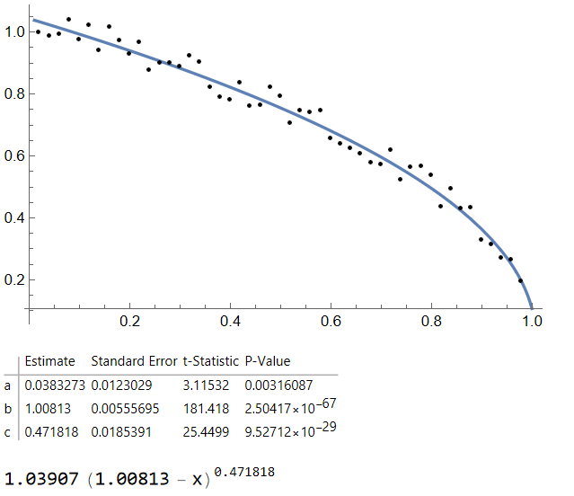
In[287]:= {min, vals} = bestFit[data]

(* Out[287]= {0.0842183, {a -> 1.0391, b -> 1.02703, c -> 0.515608}} *)

Plot[a*(b - x)^c /. vals, {x, 0.02, 0.98}, Epilog -> Point[data]]

enter image description here

$\endgroup$
2
  • $\begingroup$ Can you explain a bit more about how you deal with the b within the logarithm? I could not understand it from your code. $\endgroup$ Commented Aug 12, 2023 at 4:26
  • $\begingroup$ @ArchismanPanigrahi The function you have is of the form y=a*(b-x)^c. Taking logs of both sides we have (ignoring that log is multivalued) log(y)=log(a)+c*log(b-x). So I defined a function I call logx (not ideal naming) that, given a value b and a list vals, computes the set ov values Log[b-vals]. I use this in the objective to minimize, where the list xvals comes from the input data and b is one of the parameters we need to determine in our (best-fit) optimization. $\endgroup$ Commented Aug 12, 2023 at 16:53
3
$\begingroup$

The cause for the errors is that you give a starting value for b that is too small. You need to give a starting value for b larger than Max[data[[All,1]] otherwise you end up with complex numbers. It also doesn't hurt to put in that explicit condition.

SeedRandom[12345];
data = N[Table[{n/50, Sqrt[1 - n/50] + RandomReal[]/10}, {n, 1, 49}]]

fit = NonlinearModelFit[data, {a (b - q)^c, b > Max[data[[All, 1]]]}, 
  {{a, 0.8}, {b, Max[data[[All, 1]]]}, {c, 0.6}}, q]

NonlinearModelFit result

$\endgroup$
2
$\begingroup$

A minor variant:

d = N[Table[{n/50, Sqrt[1 - n/50] + RandomReal[]/10}, {n, 1, 49}]];
td = {#1, Log@#2} & @@@ d;
n = NonlinearModelFit[td, a + c Log[b - x], {a, b, c}, x];
Plot[Exp[n[x]], {x, 0.01, 1}, Epilog -> Point[d]]
n["ParameterTable"]
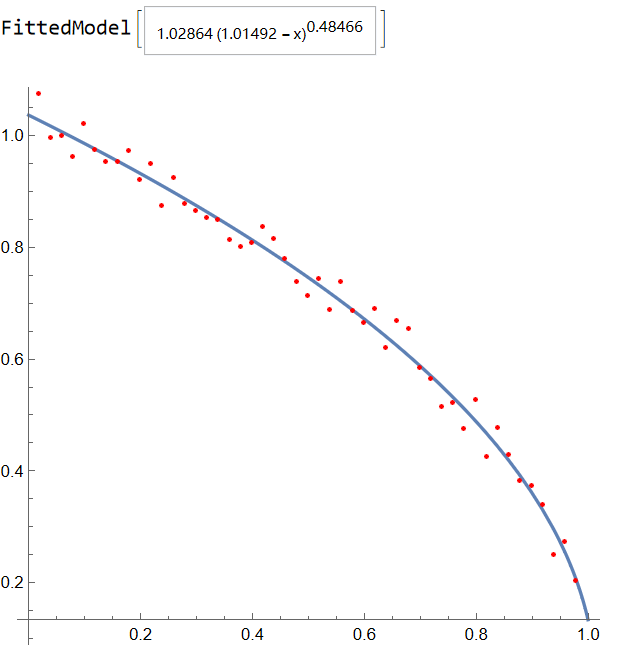
model = Exp[a] (b-x)^c /. n["BestFitParameters"]

enter image description here

$\endgroup$
2
  • $\begingroup$ Can you please explain why you used td, and the meaning of the syntax td = {#1, Log@#2} & @@@ d; ? $\endgroup$ Commented Aug 14, 2023 at 21:14
  • $\begingroup$ td is just transforming the data from {{x1,y1}, …} to {{x1, ln(y1)},…}. The @@@ just applies preceding function to all elements of list. The # are slots. $\endgroup$
    – ubpdqn
    Commented Aug 14, 2023 at 23:41

Your Answer

By clicking “Post Your Answer”, you agree to our terms of service and acknowledge you have read our privacy policy.

Not the answer you're looking for? Browse other questions tagged or ask your own question.