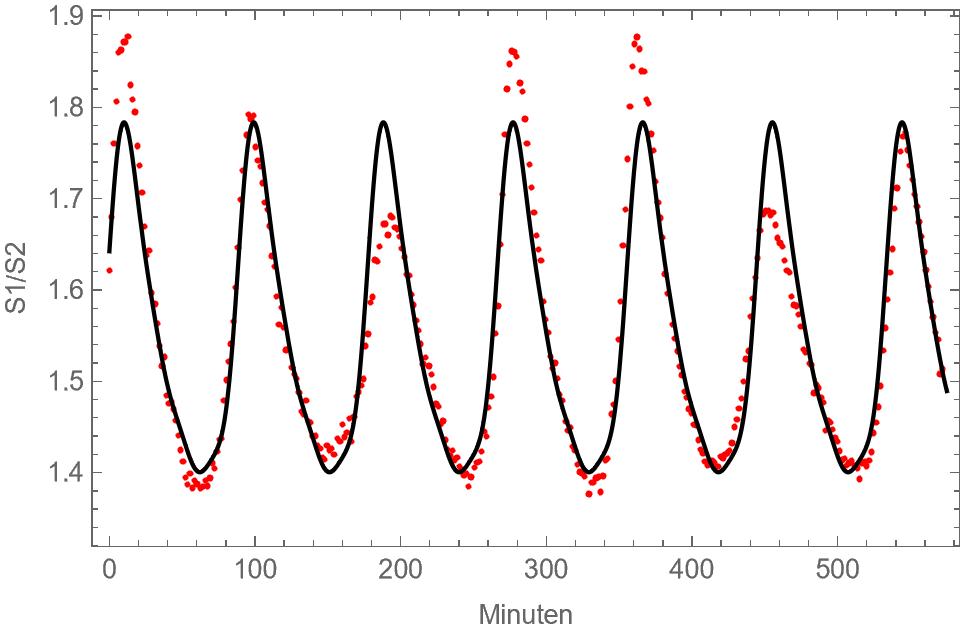
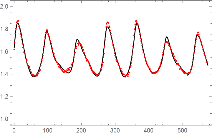
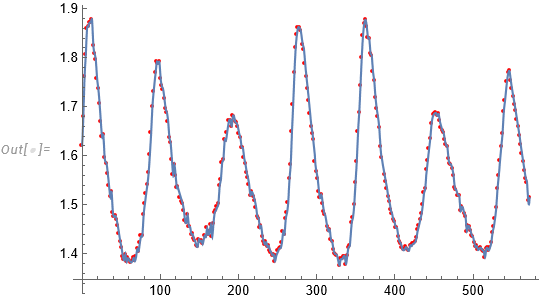
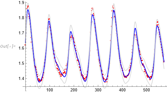
I'm trying to appropriately fit a fourier model to experimental data. But the problem is that the resulting fit doesn't consider the varying local maxima of the data.
Here's the data:
data={{0., 1.62103}, {1.59924, 1.67994}, {3.19848, 1.76026}, {4.79772,
  1.80673}, {6.39696, 1.8598}, {7.9962, 1.86282}, {9.59544,
  1.87166}, {11.2114, 1.87156}, {12.7939, 1.87728}, {14.4099,
  1.82449}, {15.9925, 1.80886}, {17.5918, 1.79485}, {19.191,
  1.75784}, {20.807, 1.73654}, {22.4062, 1.70686}, {24.0054,
  1.66943}, {25.6047, 1.63784}, {27.2039, 1.64295}, {28.8032,
  1.59652}, {31.3354, 1.58473}, {32.9346, 1.56336}, {34.5339,
  1.53878}, {36.1331, 1.51662}, {37.749, 1.52651}, {39.3483,
  1.48455}, {40.931, 1.47545}, {42.5468, 1.47792}, {44.1461,
  1.46984}, {45.7454, 1.45691}, {47.3612, 1.44064}, {48.9606,
  1.42462}, {50.5598, 1.41207}, {52.159, 1.39475}, {53.7583,
  1.38704}, {55.3575, 1.39879}, {56.9568, 1.38317}, {58.556,
  1.39112}, {60.1552, 1.38762}, {62.7207, 1.38232}, {64.3201,
  1.38509}, {65.9026, 1.39164}, {67.5019, 1.38518}, {69.1011,
  1.39424}, {70.6838, 1.41042}, {72.283, 1.40475}, {73.8823,
  1.4228}, {75.4815, 1.43597}, {77.0808, 1.43705}, {78.6967,
  1.47911}, {80.2792, 1.5015}, {81.8952, 1.52173}, {83.4944,
  1.54084}, {85.1103, 1.56518}, {86.7096, 1.60301}, {88.3255,
  1.64637}, {89.9248, 1.69936}, {91.5073, 1.73079}, {94.0729,
  1.76966}, {95.6722, 1.79222}, {97.2714, 1.78713}, {98.8706,
  1.79135}, {100.47, 1.75675}, {102.069, 1.74179}, {103.668,
  1.73523}, {105.268, 1.71698}, {106.867, 1.69583}, {108.466,
  1.68806}, {110.049, 1.67025}, {111.648, 1.63703}, {113.247,
  1.626}, {114.846, 1.59278}, {116.446, 1.56201}, {118.045,
  1.58105}, {119.644, 1.55918}, {121.244, 1.53408}, {122.843,
  1.53606}, {125.392, 1.51481}, {126.991, 1.5071}, {128.607,
  1.50275}, {130.189, 1.48783}, {131.789, 1.46677}, {133.388,
  1.46361}, {134.987, 1.47924}, {136.586, 1.45564}, {138.169,
  1.45476}, {139.768, 1.43951}, {141.367, 1.44018}, {142.983,
  1.42988}, {144.599, 1.42606}, {146.199, 1.41682}, {147.781,
  1.41454}, {149.38, 1.42971}, {150.963, 1.42491}, {152.562,
  1.42664}, {154.162, 1.42002}, {156.71, 1.43735}, {158.31,
  1.43401}, {159.909, 1.4527}, {161.508, 1.43911}, {163.107,
  1.4441}, {164.723, 1.45954}, {166.323, 1.4343}, {167.922,
  1.46126}, {169.504, 1.48359}, {171.104, 1.48829}, {172.703,
  1.49519}, {174.302, 1.50245}, {175.901, 1.53872}, {177.517,
  1.55181}, {179.117, 1.58608}, {180.716, 1.59239}, {182.315,
  1.633}, {183.914, 1.63106}, {185.514, 1.64767}, {188.062,
  1.67233}, {189.662, 1.67241}, {191.244, 1.66006}, {192.844,
  1.68123}, {194.443, 1.67911}, {196.042, 1.6684}, {197.658,
  1.66663}, {199.257, 1.65853}, {200.857, 1.64544}, {202.472,
  1.63608}, {204.072, 1.61669}, {205.654, 1.61556}, {207.254,
  1.59515}, {208.853, 1.58351}, {210.452, 1.56633}, {212.051,
  1.55562}, {213.651, 1.54092}, {215.25, 1.51884}, {216.866,
  1.52626}, {219.431, 1.51675}, {221.03, 1.50742}, {222.63,
  1.49369}, {224.212, 1.47495}, {225.812, 1.47253}, {227.411,
  1.45261}, {229.01, 1.45637}, {230.609, 1.43563}, {232.225,
  1.42526}, {233.808, 1.41891}, {235.407, 1.42398}, {236.99,
  1.4137}, {238.606, 1.41656}, {240.205, 1.40668}, {241.804,
  1.40326}, {243.387, 1.39673}, {244.986, 1.39886}, {246.585,
  1.38496}, {248.184, 1.39534}, {250.75, 1.40539}, {252.349,
  1.41112}, {253.948, 1.41193}, {255.548, 1.42339}, {257.147,
  1.44511}, {258.746, 1.43922}, {260.329, 1.4712}, {261.928,
  1.48333}, {263.544, 1.50475}, {265.127, 1.55252}, {266.726,
  1.58253}, {268.325, 1.64951}, {269.924, 1.7048}, {271.524,
  1.77026}, {273.106, 1.82019}, {274.705, 1.84745}, {276.305,
  1.8618}, {277.887, 1.86067}, {279.487, 1.85571}, {282.052,
  1.82686}, {283.651, 1.8172}, {285.251, 1.78734}, {286.85,
  1.76062}, {288.432, 1.73714}, {290.032, 1.71213}, {291.631,
  1.68495}, {293.247, 1.65939}, {294.829, 1.64458}, {296.429,
  1.6325}, {298.045, 1.58712}, {299.627, 1.5676}, {301.243,
  1.55351}, {302.842, 1.52739}, {304.442, 1.51368}, {306.041,
  1.52018}, {307.657, 1.50288}, {309.239, 1.48562}, {310.839,
  1.47884}, {313.404, 1.45589}, {315.003, 1.44615}, {316.603,
  1.44958}, {318.202, 1.42828}, {319.801, 1.42421}, {321.417,
  1.40902}, {323., 1.40048}, {324.599, 1.39907}, {326.182,
  1.39556}, {329.397, 1.37646}, {330.996, 1.38923}, {332.595,
  1.38914}, {334.178, 1.39418}, {335.777, 1.39506}, {337.393,
  1.37884}, {338.992, 1.39638}, {340.592, 1.41348}, {342.191,
  1.41578}, {344.74, 1.46429}, {346.339, 1.47461}, {347.938,
  1.50045}, {349.521, 1.54545}, {351.137, 1.58719}, {352.736,
  1.64857}, {354.335, 1.68838}, {355.934, 1.74357}, {357.534,
  1.80062}, {359.133, 1.8446}, {360.732, 1.86921}, {362.331,
  1.87709}, {363.914, 1.86407}, {365.53, 1.83981}, {367.129,
  1.83959}, {368.728, 1.80868}, {370.328, 1.80399}, {371.927,
  1.77087}, {373.51, 1.75285}, {375.109, 1.71898}, {376.708,
  1.69569}, {378.307, 1.67887}, {379.907, 1.65734}, {381.522,
  1.61742}, {383.122, 1.596}, {386.703, 1.56191}, {388.303,
  1.54718}, {389.902, 1.53308}, {391.501, 1.51604}, {393.084,
  1.50679}, {394.7, 1.48916}, {396.299, 1.48208}, {397.898,
  1.46974}, {399.497, 1.4646}, {401.097, 1.45299}, {402.696,
  1.45232}, {404.279, 1.43553}, {405.878, 1.42497}, {407.477,
  1.42119}, {409.06, 1.41202}, {410.659, 1.40749}, {412.258,
  1.40855}, {413.857, 1.41359}, {415.457, 1.41076}, {417.989,
  1.40651}, {419.588, 1.41757}, {421.187, 1.41581}, {422.787,
  1.41994}, {424.386, 1.42134}, {425.968, 1.42441}, {427.568,
  1.43257}, {429.184, 1.44978}, {430.8, 1.45837}, {432.382,
  1.47002}, {433.981, 1.48139}, {435.581, 1.49949}, {437.18,
  1.52456}, {438.779, 1.53323}, {440.378, 1.5712}, {441.978,
  1.59066}, {443.56, 1.61338}, {445.143, 1.6351}, {446.759,
  1.66504}, {449.324, 1.68336}, {450.924, 1.68639}, {452.523,
  1.68708}, {454.139, 1.6813}, {455.738, 1.68519}, {457.337,
  1.67114}, {458.936, 1.65698}, {460.519, 1.65152}, {462.102,
  1.64747}, {463.701, 1.63251}, {465.3, 1.62152}, {466.899,
  1.61931}, {468.499, 1.59303}, {470.098, 1.58356}, {471.681,
  1.58228}, {473.28, 1.57347}, {474.879, 1.56006}, {476.478,
  1.53452}, {478.061, 1.53139}, {480.643, 1.51941}, {482.226,
  1.51783}, {483.825, 1.48705}, {485.424, 1.4959}, {487.007,
  1.49279}, {488.623, 1.48235}, {490.222, 1.47662}, {491.805,
  1.44583}, {493.404, 1.45701}, {495.02, 1.4549}, {496.619,
  1.44729}, {498.201, 1.4378}, {499.801, 1.43419}, {501.4,
  1.42368}, {502.999, 1.41367}, {504.599, 1.41577}, {506.198,
  1.40778}, {507.78, 1.41046}, {509.38, 1.41262}, {511.945,
  1.40732}, {513.544, 1.40493}, {515.144, 1.393}, {516.743,
  1.41062}, {518.342, 1.41157}, {519.941, 1.40709}, {521.524,
  1.41336}, {523.123, 1.42273}, {524.722, 1.44338}, {526.305,
  1.45494}, {527.904, 1.47173}, {529.504, 1.49501}, {531.103,
  1.53354}, {532.685, 1.55843}, {534.285, 1.58945}, {535.884,
  1.61907}, {537.483, 1.64483}, {539.066, 1.68931}, {540.682,
  1.71184}, {543.231, 1.75192}, {544.813, 1.76839}, {546.429,
  1.77242}, {548.028, 1.75339}, {549.611, 1.73661}, {551.21,
  1.72117}, {552.809, 1.7048}, {554.392, 1.6911}, {555.991,
  1.67447}, {557.591, 1.65868}, {559.207, 1.64152}, {560.789,
  1.62177}, {562.372, 1.6041}, {563.988, 1.58738}, {565.587,
  1.57031}, {567.186, 1.55374}, {568.802, 1.54545}, {570.401,
  1.50809}, {572.001, 1.51358}}
And here's what I've tried so far:
k=4
modelK = a0 +
   Sum[b[i]*Sin[2*Pi*i*t/P] + d[i]*Cos[2*Pi*i*t/P], {i, 1, k}];
paramsK =
  Join[{a0}, Table[b[i], {i, 1, k}], Table[d[i], {i, 1, k}], {P}];
B[t_] = FindFit[data, {modelK, {85 < P < 90}},
  paramsK, t]
fitPlotK =
  Plot[modelK /. B[t], {t, 0, 575}, PlotStyle -> Black, Frame -> True];
The parameter P got specified to as close to the literary value as possible
Plotting the fitted model and the data it looks like this:
Now the question is how to modify the model or initial parameters for the fit to better resemble the experimental data.
Any help is greatly appreciated :D


