28
$\begingroup$

I am writing an algorithm that finds the center of 500 x 500 pixels images coming from a live feed from a camera at 50 Hz. So it has to be quick! The images are images of an optical field which looks like a "flower" (example below) which is somehow circular, so it does have a true center, but since it jiggles and it rotates, I have to calculate the true center for every frame.

Here is an example of the field:
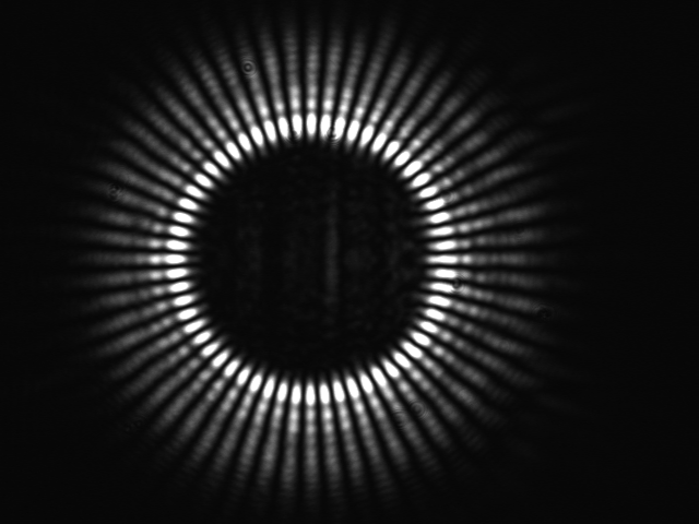
example of kernel $K$

What I did so far:

Prior to the beginning of frame capture, I prepare in advance 10 matrices $M_i$ of size 600 x 600 like this:

     linepoints[a_] := {{Cos[a], Sin[a]}, {Cos[a + Pi], Sin[a + Pi]}}
      img[l_, k_] := Graphics[{Table[Line[linepoints[a + k*Pi/(10l)]], {a, 0, 2Pi, Pi/l}],
                          White, Disk[{0, 0}, .2]}, ImageSize -> {600, 600}]
      M[l_, k_] := ImageData[ColorConvert[img[l, k], "Grayscale"], "Bit"]
      masks = mask[l, Range[10]];

The matrices in masks have all $2l$ lines going out from the center, and they are rotated of $\frac{2\pi}{10l}k$ from one another, so that $M(l,1)=M(l,11)$. Here's one for $l=30$ (so 60 rays):
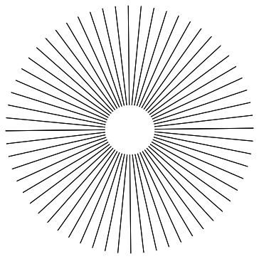
Example of $M_k$ mtrix

It is important that the number of "rays" in the $M_k$ matrices matches the number of "petals" in the true image from the camera, which is not a problem, as that number is fixed from the beginning. The algorithm calculates the discrete convolution of all 10 matrices $M_k$ with a kernel $K$ (the actual frame coming from the camera, cropped at 500 x 500 around a "guessed" center), so that I end up with a tensor $T$ made of 10 matrices of size 100 x 100.

    array = ImageData[image, "Real32"][[All, All, 2]] (*10 msec*)
    T=ListCorrelate[array, 1 - #] & /@ masks          (*about 250 msec*)

(Here image is the image in 1, not yet a frame from the video feed.) With Transpose[] I turn $T$ into a 100 x 100 matrix convol of lists of length 10, on which I run a simple visibility test:

    visibility[list_]:=(Max[list]-Min[list])/(Max[list]+Min[list])
    m = Map[visibility,convol,{2}];                   (*10 msec*)
    {x,y}=Position[m,Max[m]];                         (*0.1 msec*)

Here m is nothing else than an map of where the visibility is highest, which corresponds to the true center of the pattern. Below, the corresponding ArrayPlot[m] and ArrayPlot[Log[m]] for the optical field in Fig. 1.
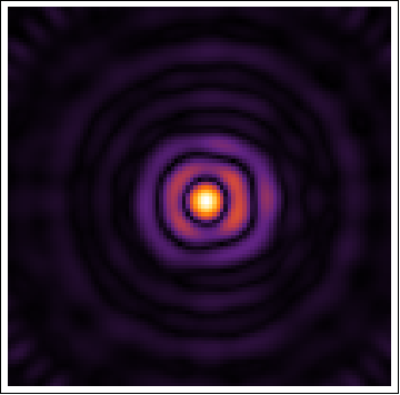
m<code>Log[m]</code>

All this is fine, except that if I use ListConvolve[] it takes 300 milliseconds per frame, while if I use the convolution theorem with FFT it takes 150 milliseconds on my 8-core machine, and to run in real-time it should take no more than 20 milliseconds. As of now, the algorithm is an order of magnitude slower than I would like it to be.

My question is the following: I have GTX 660 Ti, with 1344 CUDA cores. Is there a way I can use it to speedup the above algorithm (or a better version of it) and have it run in real-time? Or, is there a more clever version than the algorithm above? (I'm pretty sure that I am being a very naive programmer...)

EDIT

It is very important to find the center with high precision, because then by addressing the visibility curve (the plot of the 10 points calculated at the true center) I can detect rotations of the pattern with a precision even below $\pi/10l$.

I tried CUDAImageConvolve[], but it gives error messages for a too large kernel... Unfortunately a kernel is too large already around 60 x 60.

Other test images:

40 petals: https://i.sstatic.net/ktps4.png

80 petals: https://i.sstatic.net/MUAAo.png

100 petals: https://i.sstatic.net/WBiZD.png

120 petals: https://i.sstatic.net/uFlBH.png

140 petals: https://i.sstatic.net/1B3P2.png

160 petals: https://i.sstatic.net/ZKyxa.png

$\endgroup$
9
  • $\begingroup$ Is the brightness always symmetrically distributed (as in the sample image you showed)? Then you could just calculate the center of mass of the (possibly thresholded or binarized) image. That's an O(N) operation instead of O(N Log(N)) for the FFT version. $\endgroup$ Commented Apr 17, 2013 at 6:56
  • $\begingroup$ Yes, I tried, that's actually how I do the initial guessing of the center for the cropping. But then I need very high precision, as you can see from fig [3] and [4] there are circles of very low visibility just around the true center $\endgroup$
    – Ziofil
    Commented Apr 17, 2013 at 7:01
  • $\begingroup$ Notice a sort of related question: Counting radial ridges on an image $\endgroup$ Commented Apr 17, 2013 at 7:46
  • $\begingroup$ I would find it helpful if you were to attach or upload perhaps half a dozen test images, so that I might see if my parameters are at all robust. $\endgroup$
    – Mr.Wizard
    Commented Apr 17, 2013 at 8:07
  • 1
    $\begingroup$ you can also check the answer of @Jens to this question about finding Symmetry Axes of images. mathematica.stackexchange.com/questions/17060/… $\endgroup$
    – s.s.o
    Commented Apr 17, 2013 at 10:18

3 Answers 3

18
$\begingroup$

EDIT: graphical alignment issue corrected.

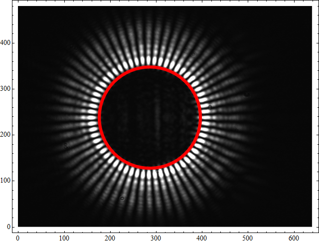
I think this has promise. The centering is almost perfect, and while the code may not be well tuned or optimized it is quite fast: 0.008736 seconds on my machine.

It works by attempting to find the center of each white "blob" and then averaging those positions.

img = Import["https://i.sstatic.net/i050B.png"];

center =
  Mean[Mean /@ 
    N@GatherBy[ArrayRules@MorphologicalComponents@MinFilter[Binarize[img, 0.99], 1], 
       Last][[;; -2, All, 1]]
  ] // Reverse;

Graphics[
 {Raster @ ImageData @ img,
  {Red, Thickness[.01], Circle[center, 110]}},
 Frame -> True]

enter image description here

$\endgroup$
3
  • $\begingroup$ If the result of a fast algorithm is close enough to the true center, i could use this to make the initial guess and then reduce the convolution to, say, a 10 x 10 instead of a 100 x 100 matrix of results. Looking forward to trying it at work in the morning! $\endgroup$
    – Ziofil
    Commented Apr 17, 2013 at 7:33
  • $\begingroup$ @Ziofil I think this is more accurate than I thought; there seems to be a graphics alignment issue in play that is causing a larger error than the code. Working on it now! $\endgroup$
    – Mr.Wizard
    Commented Apr 17, 2013 at 7:37
  • 2
    $\begingroup$ @Ziofil issue corrected; please see update! $\endgroup$
    – Mr.Wizard
    Commented Apr 17, 2013 at 7:41
18
$\begingroup$

Your image:

img = Import["https://i.sstatic.net/i050B.png"];

Here is the circle's radius and center:

crcl = ComponentMeasurements[RegionBinarize[Dilation[img, 3], 
       {{320, 240}}, 0.3], {"Centroid", "EquivalentDiskRadius"}]; // AbsoluteTiming
crcl
{0.126007, Null}
{1 -> {{284.448, 241.873}, 109.256}}

And here how precise it is:

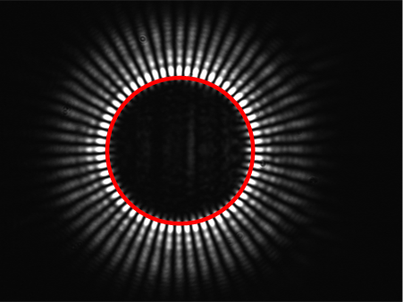
Show[img, Graphics[{Red, Thickness[.01], Circle @@@ crcl[[All, 2]]}]]

enter image description here

$\endgroup$
5
  • $\begingroup$ Vitaly, what about the timing? $\endgroup$
    – Yves Klett
    Commented Apr 17, 2013 at 6:53
  • $\begingroup$ That's a really neat solution! At the moment I'm at home and I don't have Mathematica 9, only 8, and I cannot test it. I'm afraid, though, that the point that is found does not always correspond to the highest-visibility point. $\endgroup$
    – Ziofil
    Commented Apr 17, 2013 at 6:59
  • $\begingroup$ @Ziofil I guess you should test it against your results. Also you can tweak image processing functions and parameters. $\endgroup$ Commented Apr 17, 2013 at 7:02
  • $\begingroup$ I will first thing in the morning! thank you $\endgroup$
    – Ziofil
    Commented Apr 17, 2013 at 7:04
  • $\begingroup$ @YvesKlett added - about 0.12 seconds $\endgroup$ Commented Apr 17, 2013 at 7:13
15
$\begingroup$

All the image samples you posted are basically lines pointing towards a common center. We can turn that into a simple mathematical model: Let's say every gradient in the image is normal to a line pointing towards the center. Find the center with the least squared error. So the error term would be:

squaredError = ({cx - x, cy - y}.{gx, gy})^2;

where cx/cy is the center we're looking for, x/y is the position of the respective pixel and gx/gy is the gradient at that location. Using the absolute gradient also gives less weight to pixels with low gradient strength.

Setting the derivative of this error to 0 yields a linear system:

errDerivative = Expand[D[squaredError, {{cx, cy}}]]; 
linearSystem = {{D[errDerivative, cx], 
    D[errDerivative, cy]}, -errDerivative /. {cx -> 0, cy -> 0}}

Ouput:

{{{2 gx^2, 2 gx gy}, {2 gx gy, 2 gy^2}}, {2 gx^2 x + 2 gx gy y, 2 gx gy x + 2 gy^2 y}}

So all we have to do is replace gx,gy,x,y with the actual values from the image, take the total over all pixels and solve the resulting 2x2 linear system:

img = Import["https://i.sstatic.net/MUAAo.png"];
gradientX = ImageData@GaussianFilter[img, 1, {0, 1}];
gradientY = ImageData@GaussianFilter[img, 1, {1, 0}];
xArr = Array[N[#2] &, Dimensions[gradientX]];
yArr = Array[N[#1] &, Dimensions[gradientX]];
ls = Total[
   linearSystem /. {gx -> gradientX, gy -> gradientY, x -> xArr, 
     y -> yArr}, {-2, -1}];
center = LinearSolve @@ ls;

One final correction to turn indices to coordinates:

center[[2]] = Length[gradientX] - center[[2]];

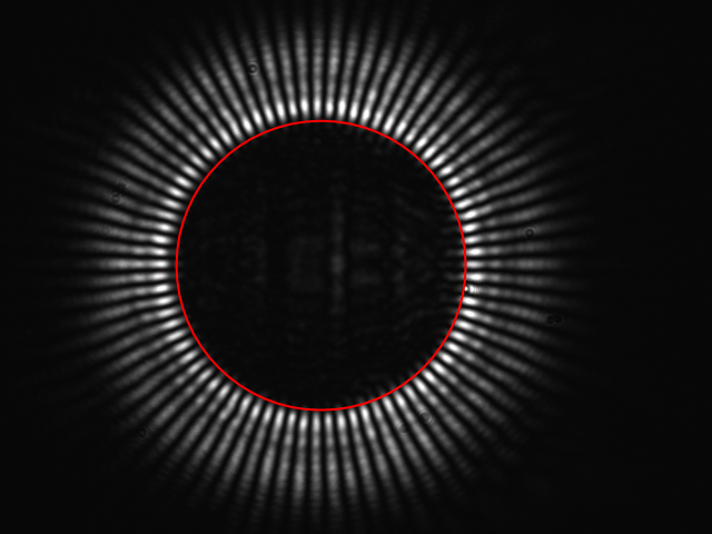
And we have the center of the flower:

Show[img, Graphics[{Red, Circle[center, Thick, 130]}]]

enter image description here

The running time on my PC is about 0.06s, but: all of the operations are simple convolution/arithmetic operations. It should be relatively easy to turn this into a C or CUDA algorithm.

Possible improvements:

  • Use a robust error function instead of least squared errors. This would lead to an interative algorithm
  • If you have an initial guess for the center, you can use that to put more "weight" on the gradients that point roughly in that direction.
  • The simple replacement calculation used above calculates gx^2, gy^2, gx*gy multiple times. This could obviously be made faster simply by calculating them only once.
$\endgroup$

Your Answer

By clicking “Post Your Answer”, you agree to our terms of service and acknowledge you have read our privacy policy.

Not the answer you're looking for? Browse other questions tagged or ask your own question.