14
$\begingroup$

I'd like (together with a few people) to prepare a presentation about Fourier series for middle/high school students. I thought it might be quite cool to play a violin sound from, say, a WAV file, then approximate it by the first one, two, three etc. terms of the corresponding Fourier series. Assuming that I have the WAV file (and it is just one note with known frequency), how could I do this?

This can be distilled to two problems: (1) transforming WAV to a list of data (and that is the easy part) and (2) finding the Fourier series of the function, whose sample is that list.

AFAIK, FourierSeries expects a function and not a list, and it seems that Fourier won't help me here. I could transform the list into a function by writing a function doing, say, linear interpolation of the data in the list by hand, but this seems overly complicated.

Any ideas?

$\endgroup$

3 Answers 3

9
$\begingroup$

Read in the wave file (use Import). Then use the Fourier[]function. This breaks it into a sum of complex exponentials. You can turn this into a trigonometric series using Euler's formula. Here's a bit more detail.

Reading in the .wav file is easy:

q = Import[fullFileName];

Now q has two parts: the data in q[[All,1]] and the sampling rate in q[[1,2]] which is in samples per second. You'll need both of these. In my case, it's the sound of a gong so I call it:

gongData = q[[All,1]];
gongTs = q[[1,2]];

(If your file is stereo, you will have to play with gongData to get it to be a single vector). Now do the FFT and plot

numSam = Length[gongData];
freqInd = 1/(gongTs numSam);
fftGongData = 
RotateLeft[Fourier[gongData, FourierParameters -> {1, -1}], 
    Round[numSam/2]];
ssf = freqInd Range[-numSam/2, numSam/2 - 1];
ListPlot[Transpose[{ssf, Abs[fftGongData]}] , PlotRange -> All, 
   Filling -> Axis, PlotLabel -> "Spectrum of the gong sound"]

ssf is a vector used to scale the horizontal axis do that it is in Hz. The plot shows the magnitude (Abs[ ]) of the sinusoidal component (i..e, the complex exponential) at each frequency.

If you want to represent this in the Cos[ ] + I Sin[ ] form instead of magnitude and phase, you can use the ExpToTrig function. For example, each of the numbers in fftGongData[[n]] represents a (complex valued) sinusoid at frequency ssf[[n]]. So, letting

w = fftGongData[[n]];
f = ssf[[n]];

this harmonic (or partial) of the sound is, into trig form,

Abs[w] Cos[2 f \[Pi] + Arg[w]] + I Abs[w] Sin[2 f \[Pi] + Arg[w]]

This is one term of the desired Fourier Series. Gather all the terms together and you have a complete representation of the signal in terms of its sinusoidal components.

$\endgroup$
8
$\begingroup$

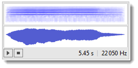
You can use direct Fourier and then feed just part of the result to InverseFourier. This is the sound of violin:

snd = ExampleData[{"Sound", "Violin"}]

enter image description here

These are data behind the sound file (it'll be the same for imported .WAV file):

dat = snd[[1, 1, 1]];

This is the sampling rate

sr = snd[[1, 2]]

22050

This is direct Fourier transform of data:

f = Fourier[dat];

To keep duration of sound the same, when we take less Fourier harmonics we need to reduce the sampling rate proportionally:

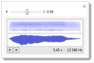
Manipulate[
  Sound[SampledSoundList[{Re@InverseFourier[
  Take[f, {1, Round[k Length[f]]}]]}, Round[k sr]]], 
{k, .001, 1, Appearance -> "Labeled", ImageSize -> Small},
FrameMargins -> 0]

enter image description here

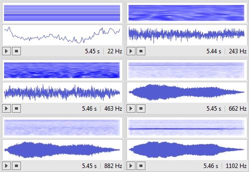
k means fraction of harmonics taken to reconstruct the sound. I am taking real part of reconstructed signal. I actually like how it sounds. This is animation of how you are adding harmonics.

enter image description here

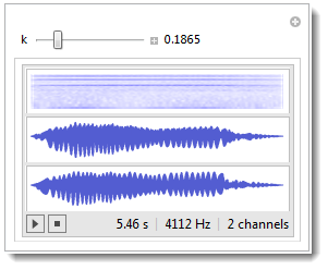
Now a very neat stereo effect (perhaps quite artificial) is when we put real and imaginary parts into different channels. At some settings a very cool stereo feel can be heard - like hear:

Manipulate[
 Sound[SampledSoundList[{Re[#], Im[#]} &[
    InverseFourier[Take[f, {1, Round[k Length[f]]}]]], 
   Round[k sr]]], {{k, .1865}, .001, 1, Appearance -> "Labeled", 
  ImageSize -> Small}, FrameMargins -> 0]

enter image description here

The imaginary part will be zero when sound is fully reconstructed at k=1.

$\endgroup$
2
  • 1
    $\begingroup$ Thanks! Is it possible to export this as a WAV file? I did try Export["file.wav",...], whith various things as ... (i.e., Sound[...], SampledSoundList[...], ...), but didn't succeed. $\endgroup$
    – mbork
    Commented Apr 5, 2013 at 21:40
  • $\begingroup$ Instead of dat = snd[[1, 1, 1]]; you need dat = snd[[1, 1]];. $\endgroup$
    – Russ Lyons
    Commented Dec 26, 2017 at 2:25
5
$\begingroup$

This two-years-old question encouraged me to create a Mathematica activity for my Acoustics students, but it became so interesting, that I created SIX Mathematica activities, that start from manually ploting a spectrum, continue with importing a WAV file and approximating with a Fourier series (as was asked in this question) and finish with the complex Discrete Fourier Transform, which is the one really used (instead of Fourier series) in the processing of digital signals. Those documents can be found in the several "Acoustic Spectrum" sections in this link: http://matecmaticaacustica.weebly.com, I hope it is useful. Regards.

$\endgroup$

Your Answer

By clicking “Post Your Answer”, you agree to our terms of service and acknowledge you have read our privacy policy.

Not the answer you're looking for? Browse other questions tagged or ask your own question.