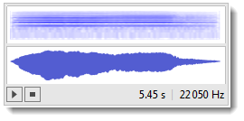
ThisYou can use direct Fourier and then feed just part of the result to InverseFourier. This is the sound of violin:
snd = ExampleData[{"Sound", "Violin"}]

These are data behind the sound file (it'll be the same for imported .WAV file):
dat = snd[[1, 1, 1]];
This is the sampling rate
sr = snd[[1, 2]]
22050
This is direct Fourier transform of data:
f = Fourier[dat];
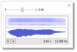
Now my gut tells me that ifTo keep duration of sound the same, when we take less Fourier harmonics we need to reduce the sampling rate proportionally:
Manipulate[
  Sound[SampledSoundList[{Re@InverseFourier[
  Take[f, {1, Round[k Length[f]]}]]}, Round[k sr]]],
{k, .001, 1, Appearance -> "Labeled", ImageSize -> Small},
FrameMargins -> 0]

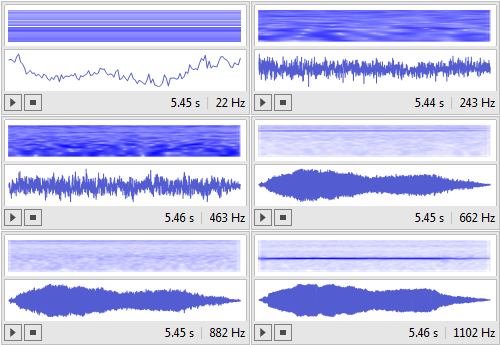
k means fraction of harmonics taken to reconstruct the sound. I am taking real part of reconstructed signal. This all maybe a bit naive but works nicely to instructively demonstrate something to non-dedicated crowd. I actually lovelike how it sounds. This is animation of how you are adding harmonics.

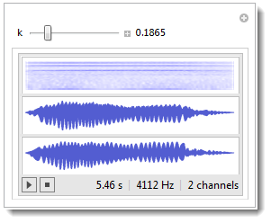
Now a very neat stereo effect (perhaps quite artificial) is when we put real and imaginary parts into different channels. At some settings a very cool stereo feel can be heard - like hear:
Manipulate[
 Sound[SampledSoundList[{Re[#], Im[#]} &[
    InverseFourier[Take[f, {1, Round[k Length[f]]}]]],
   Round[k sr]]], {{k, .1865}, .001, 1, Appearance -> "Labeled",
  ImageSize -> Small}, FrameMargins -> 0]

The imaginary part will be zero when sound is fully reconstructed at k=1.
