3D plot Versus actual values

Question

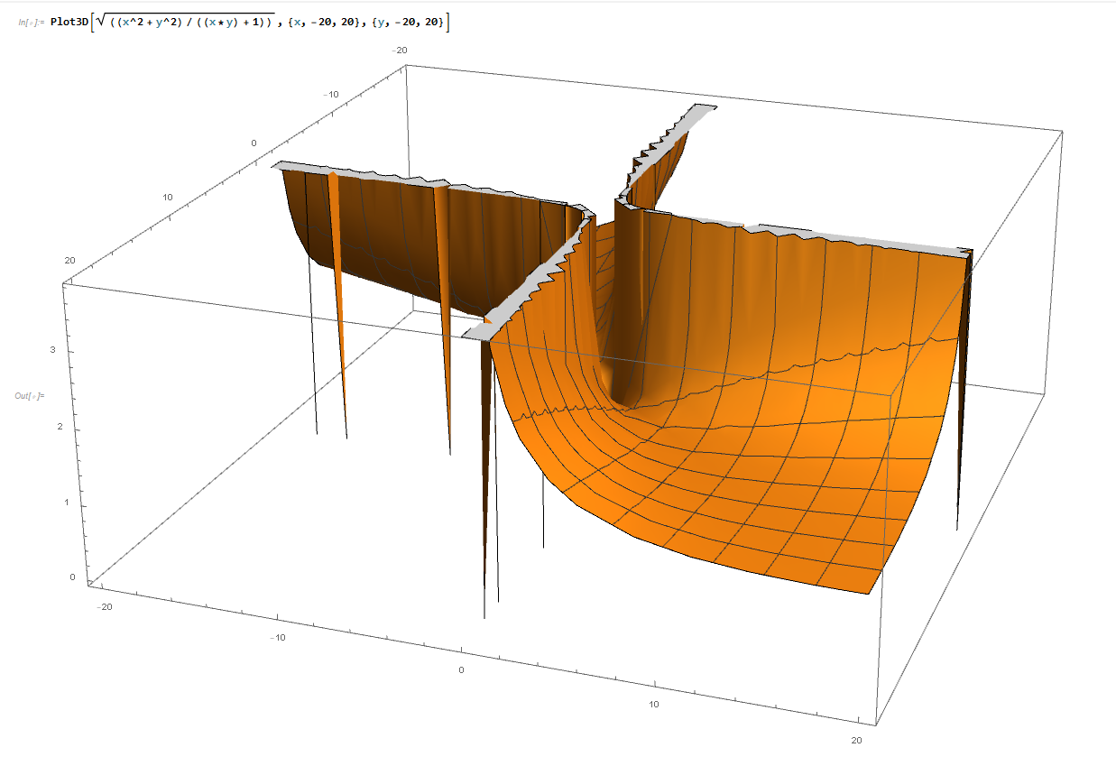
I am plotting a 3D graph as you can see:

Plot3D[Sqrt[((x^2 + y^2)/((x*y) + 1))], {x, -20, 20}, {y, -20, 20}]

Then I display the integer values of it for the same range (thanks to members here who helped me with it on this board here!) like so:

sol = SortBy[{x, y, s} /.Solve[s == Sqrt[((x^2 + y^2)/((x*y) + 1))] && -20 <= x <= 20 && -20 <= y <= 20, {x, y, s}, Integers], Last]

Now if you notice the graph only goes up to a value of 4 max (on the output values - running UP on the left side) whereas the integer solution for that range easily is going up to a value of 20 : {20, 0, 20} . So why is it that the graph is not showing anything larger than 4 here?

Also: for example the value of output of 1,20 is 4.36 but if you look at the graph, it spikes down (right in the middle, lower part of the chart near 0), instead of being at 4.36. What are all those SPIKES exactly on the chart? Why don't they map to some actual values? I wonder they are the imaginary roots?

Can we show values on the graph like local min and max?

How can I make this graph more clear to show all values or in a better readable format?

In addition, can I just plot a 3D graph of ONLY the integer values?

Thanks in Advance! Steve.

Answer 1

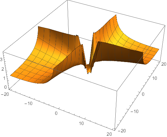
Here's the modification to @MarkR's solution I alluded to in the comments (note the Re@Sqrt[..] and the RegionFunction, both of which work together to give the right plot):

allowedValue = 
  Select[Flatten[Table[{x, y}, {x, -20, 20, 1}, {y, -20, 20, 1}], 1], 
   Times @@ # + 1 != 0 &];
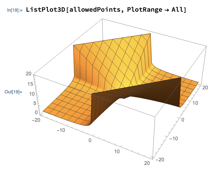
allowedPoints = 
  With[{x = #[[1]], y = #[[2]]}, {x, y, 
      Re@Sqrt[((x^2 + y^2)/((x*y) + 1))]}] & /@ allowedValue;
ListPlot3D[allowedPoints, 
 RegionFunction -> Function[{x, y, z}, x y + 1. > 0.], 
 ClippingStyle -> None]

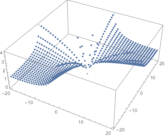
Although, the OP in a comment indicates interest in "integer-outputs only," which is interpreted to mean outputs at integer {x, y} below:

ListPointPlot3D[
 Flatten[Table[{x, y, Sqrt[((x^2 + y^2)/((x*y) + 1))]},
 {x, -20, 20, 1}, {y, -20, 20, 1}], 1]]
(* Power::infy errors which are ignored by ListPointPlot3D *)

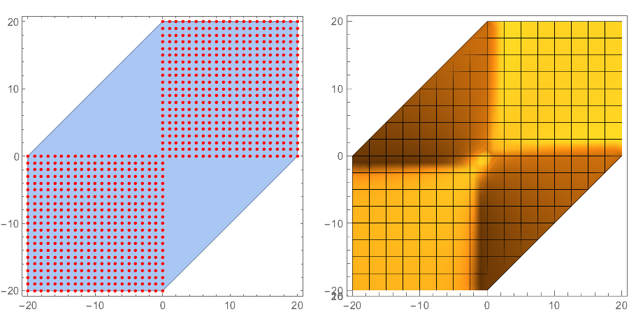
As for my convex hull remark about ListPlot3D, which I made under @MarkR's answer, ListPlot3D interpolates a surface through the points. To do that, it constructs a domain for the interpolation. The domain is the ConvexHullMesh of the xy coordinates of the data. Compare:

allowedPoints =  (* MarkR's version *)
  With[{x = #[[1]], y = #[[2]]}, {x, y, 
      Sqrt[((x^2 + y^2)/((x*y) + 1))]}] & /@ allowedValue;

realPoints = 
  Cases[allowedPoints, {x_, y_, z_ /; MatchQ[N@z, _Real]} :> {x, y}];

GraphicsRow[{
  Show[
   ConvexHullMesh[realPoints],
   Graphics[{Red, Point@realPoints}],
   Frame -> True
   ],
  ListPlot3D[allowedPoints, 
   RegionFunction -> Function[{x, y, z}, x y + 1. > 0.], 
   ClippingStyle -> None, ViewPoint -> {0, 0, Infinity}]
  }]

For some reason, adding RegionFunction -> Function[{x, y, z}, x y + 1. > 0.] to @MarkR's ListPlot3D does not exclude the sheets as it does in my code that began this answer. I guess it's because none of the real points lie in the excluded region, but I would think Mathematica could do better.

Answer 2

Use PlotRange to constrain what is plotted. Mathematica scales automatically and this may be confusing at first. You correctly checked the value to see the range making the auto-scaling more obvious.

This gives you all of the plot:

Plot3D[Sqrt[((x^2 + y^2)/((x*y) + 1))], {x, -20, 20}, {y, -20, 20}, PlotRange -> All] 

Later you said you want integers. You may get those with the following:

foo = Table[
   Sqrt[((x^2 + y^2)/((x*y) + 1))], {x, -20, 20, 1}, {y, -20, 20, 1}];
ListPlot3D[foo,PlotRange->All]

You may further wish to restrict the values of Infinity or ComplexInfinity with something like this:

allowedValue = 
  Select[Flatten[Table[{x, y}, {x, -20, 20, 1}, {y, -20, 20, 1}], 1], 
   Times @@ # + 1 != 0 &];
allowedPoints = 
  With[{x = #[[1]], y = #[[2]]}, {x, y, 
      Sqrt[((x^2 + y^2)/((x*y) + 1))]}] & /@ allowedValue;
ListPlot3D[allowedPoints]

You'll notice that you don't need the PlotRange on this last plot (identical plot if you do that).

The resulting plot: