2
$\begingroup$

Consider some data

data = {{x1,y1},{x2,y2},...}

I organize a density distribution using

datadistr = SmoothKernelDistribution[data]
PDF[datadistr, {x, y}]

I know that the real distribution must vanish at $x\leqslant x_{\text{min}}$ and, independently, $y \leqslant y_{\text{min}}, y \geqslant y_{\text{max}}$. Quantitative statement is that there are no points with $x \leqslant x_{\text{min}}, y \leqslant y_{\text{min}}, y \geqslant y_{\text{max}}$ in the data set.

However, PDF tells me that the distribution is non-zero in this domain. I do not know how to let the PDF know that the distribution must be zero in $x_{\text{min}}$ and $y_{\text{min}}, y_{\text{max}}$, i.e. to force it smoothly falls to zero close to these thresholds. Is there any way to impose this restriction?

$\endgroup$
4
  • $\begingroup$ Well, the distribution is created by convolution of the sum of Dirac-measures centered at the data points against a smoothing kernel. By construction, the resulting distribution bleeds a bit out of the bounds of the distribution from which you have sampled. (You can remedy the effect a little by picking a compactly supported smoothing kernel and by choosing a not too broad bandwidth parameter.) Maybe SmoothKernelDistribution is not the appropriate tool for what you try to do. $\endgroup$ Commented Mar 20, 2019 at 21:45
  • $\begingroup$ @HenrikSchumacher : got it. Thank you! $\endgroup$ Commented Mar 20, 2019 at 21:55
  • $\begingroup$ You're welcome. $\endgroup$ Commented Mar 20, 2019 at 21:57
  • 2
    $\begingroup$ Try the "Bounded" option when there are "hard" boundaries. $\endgroup$
    – JimB
    Commented Mar 20, 2019 at 22:27

1 Answer 1

3
$\begingroup$

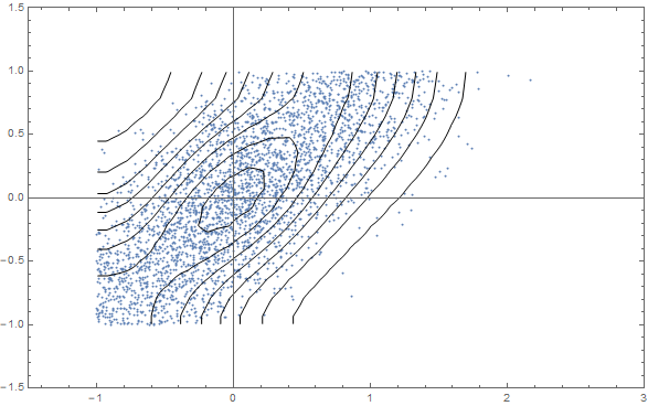
@HenrikSchumacher explained why you're getting "leakage" outside of the fixed boundaries of your data generation process. Here's one way to account for the kind of borders you have: use the "Bounded" option.

(* Generate some bounded data *)
data = RandomVariate[BinormalDistribution[{0, 0}, {1, 1}, 0.9], 5000];
data = Select[data, #[[1]] > -1 && -1 < #[[2]] < 1 &];

(* Get nonparametric density estimate *)
skd = SmoothKernelDistribution[data, 0.3, {"Bounded", {{-1, ∞}, {-1, 1}}, "Gaussian"}];

(* Show results *)
Show[ListPlot[data, PlotRange -> {{-1.5, 3}, {-1.5, 1.5}}, Frame -> True],
 ContourPlot[PDF[skd, {x, y}], {x, -1.5, 3}, {y, -1.5, 1.5},
  ContourShading -> None, PlotPoints -> 100]]

Bounded pdf and data points

And as a check see if pdf integrates to 1:

NIntegrate[PDF[skd, {x, y}], {x, -1, ∞}, {y, -1, 1}]
(* 1. *)
$\endgroup$

Your Answer

By clicking “Post Your Answer”, you agree to our terms of service and acknowledge you have read our privacy policy.

Not the answer you're looking for? Browse other questions tagged or ask your own question.