6
$\begingroup$

I'm rather new to Mathematica having been a longtime Matlab user, so apologies if my question is framed incorrectly or I have missed out expected infomation. I have tried to distill the problem to the essentials.

Effectively I am trying to plot a a transformed distribution in a similar fashion to this example code:

    data = RandomVariate[NormalDistribution[6, 5/3], 10^6];
    Show[Histogram[data, Automatic, "PDF"], 
    Plot[PDF[NormalDistribution[6, 5/3], x], {x, 0, 14}, 
    PlotStyle -> Thick]]

I have create a transformed distribution, sampled some data from it using RandomVariate and plotted it in a histogram.

    hiod = 6.5/2;
    transDistrib = 
    TransformedDistribution[hiod/Tan[theta*Degree], 
    theta \[Distributed] NormalDistribution[6, 5/3]];
    dataTrans = RandomVariate[transDistrib, 10^6];
    Histogram[dataTrans, {0, 80, 1}, "PDF", ImageSize -> Large ]

This works as expected (I have done the same thing in Matlab). However, the equivalent generation of a PDF fails (code just hangs and aborts).

    Plot[PDF[transDistrib, x], {x, 0, 80}, PlotStyle -> Thick]

I get the distinct feeling I an making a terribly simple error, either in my basic coding or understanding of how to represent probability distributions in Mathematica.

Ultimately I would like to derive the equation for the transformed distribution, but I have stumbled at this earlier stage using Mathematicas inbuilt functions.

Any pointers to solving my error would be greatly appreciated. I'm using Mathematica 11.0.1 on macOSX Sierra.

$\endgroup$
9
  • $\begingroup$ What is hiod? Here it is underfined, therefore TransformedDistribution also remains unevaluated. $\endgroup$
    – Nicholas G
    Commented Oct 23, 2016 at 12:00
  • $\begingroup$ Ah, sorry, this is an error in my post hiod is defined, and works fine with generating the histogram with the transformed distribution. I'll edit the post to correct this. Generating the PDF still fails though. $\endgroup$
    – flyingmind
    Commented Oct 23, 2016 at 12:06
  • $\begingroup$ Have edited the post to define hiod. I did this in the code, but made an error in transferring the code to the post. The histogram for the transformed distribution works fine so TransformedDistribution appears to be evaluated fine. The code hangs at the point of generating the PDF. $\endgroup$
    – flyingmind
    Commented Oct 23, 2016 at 12:10
  • $\begingroup$ Thanks. I did wonder what TransformedDistribution did internally as I could indeed get the exact same result from doing the transform myself. I assumed TransformedDistribution was doing something more clever from the examples in the help text in Mathematica. Deriving the PDF algebraically is indeed the ultimate aim. I was hoping that would come out of TransformedDistribution some way, but it sounds as if I misunderstood. $\endgroup$
    – flyingmind
    Commented Oct 23, 2016 at 12:49
  • 4
    $\begingroup$ Yes, the periodicity of Tan as @NicholasG suggests is an issue. You don't have a simple one-to-one function. You should look up "wrapped normal" to see that when you restrict the angles you're feeding to your function to range from say 0 to $\pi$ radians (or 0 to 180 degrees), the resulting density of that random variable has an infinite number of terms. But because you'll then have a one-to-one function, you can likely get an algebraic form for the density of the transformed variable but it will almost certainly have an infinite number of terms. $\endgroup$
    – JimB
    Commented Oct 23, 2016 at 15:27

2 Answers 2

3
$\begingroup$
hiod = 6.5/2;

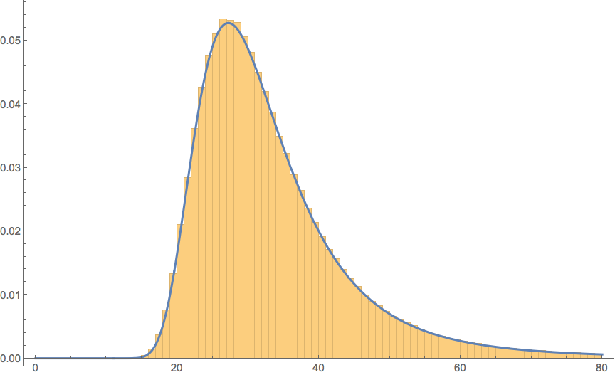
Since the tails of a normal distribution go outside of the allowed range, use TruncatedDistribution to constrain the range of theta

transDistrib = 
  TransformedDistribution[hiod/Tan[theta*Degree], 
   theta \[Distributed] 
    TruncatedDistribution[{0, 90}, NormalDistribution[6, 5/3]]];

dataTrans = RandomVariate[transDistrib, 10^6];

Show[
 Histogram[dataTrans, {0, 80, 1}, "PDF", ImageSize -> Large],
 Plot[PDF[transDistrib, x], {x, 0, 80}, PlotStyle -> Thick]]

enter image description here

EDIT:

With a different mean for the underlying NormalDistribution, the bin specification for the Histogram must be adjusted.

transDistrib = 
  TransformedDistribution[hiod/Tan[theta*Degree], 
   theta \[Distributed] 
    TruncatedDistribution[{0, 90}, NormalDistribution[3, 5/3]]];

dataTrans = RandomVariate[transDistrib, 10^6];

Show[Histogram[dataTrans, {0, 250, 1}, "PDF", ImageSize -> Large], 
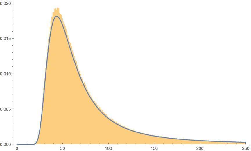
 Plot[PDF[transDistrib, x], {x, 0, 250}, PlotStyle -> Thick]]

enter image description here

$\endgroup$
8
  • $\begingroup$ Thanks, this seems to work well, but changing the mean of the normal distribution results in the histogram and the pdf giving quite different probabilities. $\endgroup$
    – flyingmind
    Commented Oct 23, 2016 at 18:26
  • $\begingroup$ hiod = 6.5/2; transDistrib = TransformedDistribution[hiod/Tan[theta*Degree], theta \[Distributed] TruncatedDistribution[{0, 90}, NormalDistribution[3, 5/3]]]; dataTrans = RandomVariate[transDistrib, 10^6]; Show[Histogram[dataTrans, {0, 80, 1}, "PDF", ImageSize -> Large], Plot[PDF[transDistrib, x], {x, 0, 80}, PlotStyle -> Thick]] $\endgroup$
    – flyingmind
    Commented Oct 23, 2016 at 18:26
  • $\begingroup$ Sorry, pressed enter too soon.... Not suite sure what the difference is here as both are being generated by transDistrib. $\endgroup$
    – flyingmind
    Commented Oct 23, 2016 at 18:27
  • $\begingroup$ @flyingmind - see edit. $\endgroup$
    – Bob Hanlon
    Commented Oct 24, 2016 at 0:38
  • 1
    $\begingroup$ For your update about 5.5% of the data lies above 250 and with the bin specification of {0,250,1}, Histogram ignores that data and causes the "bars" to show above the PDF of the transformed distribution. So I'd argue that the apparent lack of fit at the higher probability density values is a bit misleading. (In other words, your fit is better than it looks.) The same thing happens with the other histogram but only about 1.4% of the data is above 80 so the lack of fit does not look as bad. $\endgroup$
    – JimB
    Commented Oct 24, 2016 at 6:14
2
$\begingroup$

If most (meaning greater than 99.9%) of the probability is between angles of -90 and +90 degrees, then using the standard transformation of a random variable techniques (find inverse function, multiply by Jacobian, etc.) will give an "exact approximate" or "approximately exact" result. (The exact result requires dealing with a wrapped normal distribution.)

There's no mathematical problem using negative angles and if negative angles are not a problem with your experimental design, the following should work. The density function of $y=hiod/\tan{(\theta \pi/180)}$ where $\theta \sim N(\mu,\sigma)$ (and $\theta$ is in degrees) can be calculated:

μ = 6;
σ = 5/3;
hiod = 13/4;
pdf[y_, hiod_, μ_, σ_] :=
  (2 π σ^2)^(-1/2) Exp[-( (180 ArcCot[y/hiod])/π - μ)^2/(2 σ^2)]*
  180/(hiod π (1 + (y/hiod)^2))

We can take some random samples:

d = NormalDistribution[\[Mu], \[Sigma]];
z = RandomVariate[d, 10^6];
dataTrans = hiod/Tan[z*Degree];

There are many extreme values that make using the defaults for Histogram unsatisfactory so we create a custom set of bins:

lower = 0;
upper = 85;
bins = {Flatten[{Min[dataTrans], Table[i, {i, lower, upper}], Max[dataTrans]}]};
Show[Histogram[dataTrans, bins, "PDF", ImageSize -> Large,
  PlotRange -> {{lower, upper}, Automatic},
  PlotLabel -> Style["μ = 6", Bold, Large]],
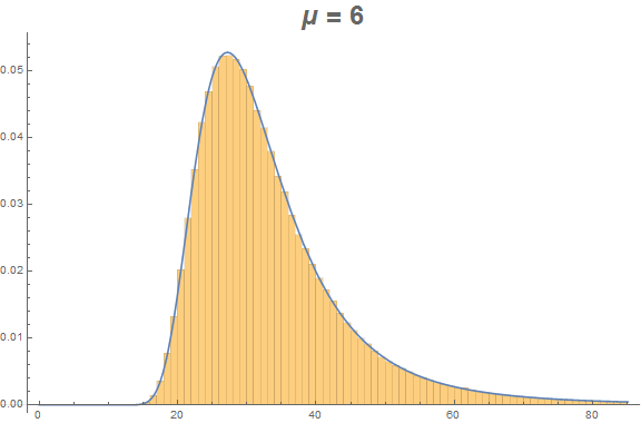
 Plot[pdf[y, hiod, μ, σ], {y, lower, upper}]]

Histogram for mean 6

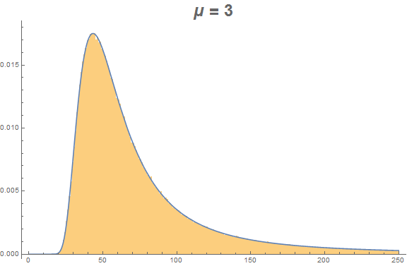
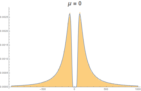
Below are the figures for μ=3 and μ=0 showing the histogram and probability density function:

Histogram for mean 3

Histogram for mean 0

$\endgroup$
2
  • $\begingroup$ Thanks. This is very nice. I am starting to like Mathematica more and more as I get use to it. I would like to work out the exact symbolic solution so have started to investigate the wrapped normal and the von Mise distributions. For my particular application negative angles would mean the eyes are pointing behind the head, and angles > 90 that the eyes are diverging. So neither is physiologically plausible, but mathematically they are fine. Similarly hoid > 0 else the distance between the eyes is zero. $\endgroup$
    – flyingmind
    Commented Oct 24, 2016 at 20:34
  • $\begingroup$ Actually hiod < 0 would be a negative distance between the eyes. $\endgroup$
    – flyingmind
    Commented Oct 24, 2016 at 20:38

Your Answer

By clicking “Post Your Answer”, you agree to our terms of service and acknowledge you have read our privacy policy.

Not the answer you're looking for? Browse other questions tagged or ask your own question.