ListLogLogPlot origin issues and numerical instability

Question

I have the following long functions f1and f2 dependent on parameters ω and g1:

f1 = (1.92`*^8 g1^2)/(10000 (1 + 40000 ω^2) + (400 + 4 ω^2) (1 + 160000 g1^4 + 40004 ω^2 + 160000 ω^4 - 800 g1^2 (-1 + 400 ω^2)) + 200 (-4 ω^2 (1 - 40000 g1^2 + 40000 ω^2) + 20 (1 + 400 g1^2 + 40000 ω^2))) + (96000.` g1^2 (400 + 4 ω^2))/(10000 (1 + 40000 ω^2) + (400 + 4 ω^2) (1 + 160000 g1^4 + 40004 ω^2 + 160000 ω^4 - 800 g1^2 (-1 + 400 ω^2)) + 200 (-4 ω^2 (1 - 40000 g1^2 + 40000 ω^2) + 20 (1 + 400 g1^2 + 40000 ω^2))) + (120200.` (10000 + 200 (20 - 4 ω^2) + (1 + 4 ω^2) (400 + 4 ω^2)))/(10000 (1 + 40000 ω^2) + (400 + 4 ω^2) (1 + 160000 g1^4 + 40004 ω^2 + 160000 ω^4 - 800 g1^2 (-1 + 400 ω^2)) + 200 (-4 ω^2 (1 - 40000 g1^2 + 40000 ω^2) + 20 (1 + 400 g1^2 + 40000 ω^2)))
f2 = (7.68`*^8 g1^2)/(160000 (1 + 40000 ω^2) + (400 + 4 ω^2) (1 + 160000 g1^4 + 40004 ω^2 + 160000 ω^4 - 800 g1^2 (-1 + 400 ω^2)) + 800 (-4 ω^2 (1 - 40000 g1^2 + 40000 ω^2) + 20 (1 + 400 g1^2 + 40000 ω^2))) + (96000.` g1^2 (400 + 4 ω^2))/(160000 (1 + 40000 ω^2) + (400 + 4 ω^2) (1 + 160000 g1^4 + 40004 ω^2 + 160000 ω^4 - 800 g1^2 (-1 + 400 ω^2)) + 800 (-4 ω^2 (1 - 40000 g1^2 + 40000 ω^2) + 20 (1 + 400 g1^2 + 40000 ω^2))) + (120200.` (160000 + 800 (20 - 4 ω^2) + (1 + 4 ω^2) (400 + 4 ω^2)))/(160000 (1 + 40000 ω^2) + (400 + 4 ω^2) (1 + 160000 g1^4 + 40004 ω^2 + 160000 ω^4 - 800 g1^2 (-1 + 400 ω^2)) + 800 (-4 ω^2 (1 - 40000 g1^2 + 40000 ω^2) + 20 (1 + 400 g1^2 + 40000 ω^2)))

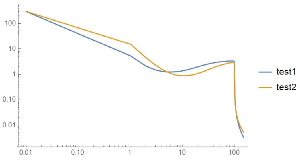
I intend to find the integral of f1 and f2 with respect to ω for varying g1 values. Then doing a Log-Log plot of the resulting integrand against g1:

test1 = Table[{g1, 1/(2 π)*NIntegrate[Evaluate[f1], {ω, -100, 100}]}, {g1, 0, 150}];
test2 = Table[{g1, 1/(2 π)*NIntegrate[Evaluate[f2], {ω, -100, 100}]}, {g1, 0, 150}];

ListLogLogPlot[{test1, test2}, PlotRange -> All, Joined -> True, PlotLegends -> {"test1", "test2"}]

I am returned with:

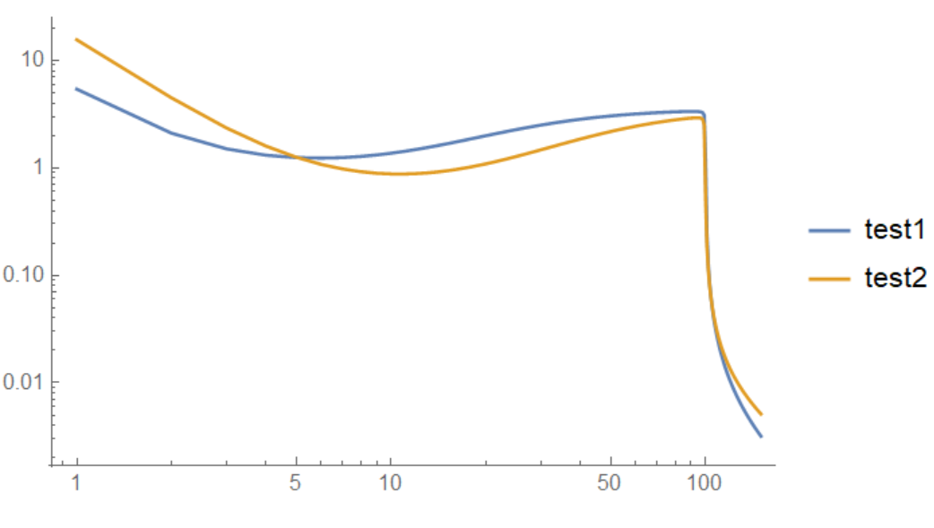
First of all it is important to me that the graph shows that they both start at the same point (which they really do). But it is clear that when the x-axis (g1) starts at 1, the two curves starts at two different y values. I was thinking maybe this is because it is not possible to show Log[0]. I tried to remedy the issue by picking a g1 value close to 0 and replot it:

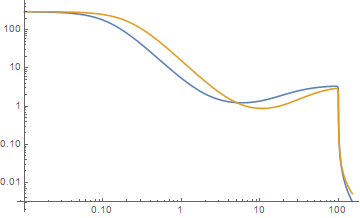
Clearly they do start from the same value when g1=0.01 but there appears to be a kink around g1=1. In general, I just want a Log-Log graph that shows that both curves starts at the same point when the x-axis is 0 How should I approach this?

Second of all, it appears that beyond g1=100 the curve drops suddenly to about 0.01. I think it might be numerical instabilities but I'm not sure what's going on here. If it were numerics, I should have had warnings but I didn't see any. What is going on here?

Answer 1

You can get a smoother result by calculating the integrals analytically (though not in closed form) first:

aux1[g1_, \[Omega]_] = Integrate[f1, \[Omega]];
aux2[g1_, \[Omega]_] = Integrate[f2, \[Omega]];

int1[g1_] = aux1[g1, 100] - aux1[g1, -100];
int2[g1_] = aux2[g1, 100] - aux2[g1, -100];

LogLogPlot[{1/(2 \[Pi]) int1[g], 1/(2 \[Pi]) int2[g]}, {g, 0.01, 150}]