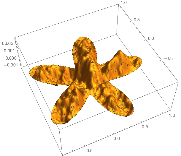
Yes, it is possible and it is also very reasonable to do so (for example in iterative schemes for nonlinear equations - building an interpolating function in between just wastes a lot of time).
One can use those facilities that NDSolve uses as backend to assemble mass and stiffness matrix and create a load vector by mass.f, where f is the vector of function values on vertices (this somewhat assumes that f represents a more or less smooth function). Afterwards, you have to deploy the boundary conditions into this load vector.
Here is a simple example, essential copied from here.
Creating a mesh:
R = DiscretizeRegion[
  BoundaryMeshRegion[
   Map[
    t \[Function] (2 + Cos[5 t])/3 {Cos[t], Sin[t]},
    Most@Subdivide[0., 2. Pi, 2000]],
   Line[Partition[Range[2000], 2, 1, 1]]
   ],
  MaxCellMeasure -> 0.00025,
  MeshQualityGoal -> "Maximal"
  ]

Suppose we'd like to solve a Poisson problem with homogeneous boundary conditions:
$$\left\{\begin{array}{rcll}
- \Delta u &= &f, &\text{in $\varOmega$},\\
u_{\partial \varOmega} &= &0. \end{array}\right.$$
Setting up a first order mesh, the pde, and discretize it.
Needs["NDSolve`FEM`"]
Rdiscr = ToElementMesh[R, "MeshOrder" -> 1];
vd = NDSolve`VariableData[{"DependentVariables",
     "Space"} -> {{u}, {x, y}}];
sd = NDSolve`SolutionData[{"Space"} -> {Rdiscr}];
cdata = InitializePDECoefficients[vd, sd,
   "DiffusionCoefficients" -> {{-IdentityMatrix[2]}},
   "MassCoefficients" -> {{1}}
   ];
bcdata = InitializeBoundaryConditions[vd, sd, {DirichletCondition[u[x, y] == 0., True]}];
mdata = InitializePDEMethodData[vd, sd];
dpde = DiscretizePDE[cdata, mdata, sd];
dbc = DiscretizeBoundaryConditions[bcdata, mdata, sd];
{load, stiffness, damping, mass} = dpde["All"];
Now, we can take a random vector f and create its associated load vector:
f = RandomVariate[NormalDistribution[], Length[mass]];
load = mass.Partition[f, 1];
DeployBoundaryConditions[{load, stiffness}, dbc];
Solving the equation with LinearSolve.
solution = LinearSolve[stiffness, load, Method -> "Pardiso"];
And plotting the result:
solfun = ElementMeshInterpolation[{Rdiscr}, solution];
Plot3D[solfun[x, y], {x, y} \[Element] R]


