Implement fractional Laplacian

Question

What is a way to implement the Fractional Laplacian with Mathematica?

How can we apply such implementation to numerically solve the problem

$$(-\Delta)^su = 1 \text{ in } B_1(0), \\ u = 0 \text{ in } \mathbb{R}^2 \setminus B_1(0), $$ where $B_1(0)$ is the unit disk centered at the origin?

Answer 1

I can provide an approach by finite elements and an application of the functional calculus of selfadjoint operators.

Background

The spectrum of the Laplacian on a bounded domain $\varOmega$ with sufficiently smooth boundary subject to homogeneous Dirichlet boundary conditions is discrete. By the spectral theorem, there are eigenfunctions $e_i \in H^1_0(\varOmega)$ and $\lambda_i \in \mathbb{R}$ with $-\Delta \, e_i = \lambda_i \, e_i$ and $0 < \lambda_1 \leq \lambda_2 \leq \dotsc$ and $$ \int_\varOmega e_i(x) \, e_j(x) \, \operatorname{d} x = \delta_{ij}. $$ By functional calculus, the solution $u \in H^{2s}(\varOmega) \cap H^{s}_0(\varOmega)$ to $(-\Delta)^s \,u = f$ for $f \in L^2(\varOmega)$ can be represented by $$u = \sum_{i=1}^\infty \left( \lambda_i^{-s} \, e_i \cdot \int_\varOmega f(x) \, e_i(x) \, \operatorname{d} x \right).$$ Weyl's law states that the eigenvalues behave as $\lambda_i \sim i^\frac{2}{\operatorname{dim}(\varOmega)}$ for $i \to \infty$. (You can get an idea of the law by performing a $\sin$-Fourier transform on the eigenvalue equation $- \Delta v = \lambda \, v$ for functions on the square $[0, 2\pi] \times [0, 2\pi]$.)

Thus, it is meaningful to use a truncated expansion in order to approximate $u$.

Our aim is now to use finite elements to approximate the eigenfunctions $e_i$ and the eigenvalues $\lambda_i$.

Implementation

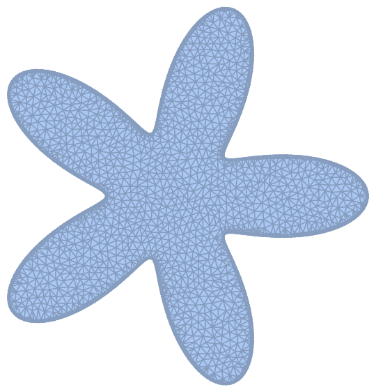
First, we create a nice domain. Disks are boring so I use the following starfish:

R = DiscretizeRegion[
  BoundaryMeshRegion[
   Map[
    t \[Function] (2 + Cos[5 t])/3 {Cos[t], Sin[t]}, 
    Most@Subdivide[0., 2. Pi, 2000]],
   Line[Partition[Range[2000], 2, 1, 1]]
   ],
  MaxCellMeasure -> 0.001,
  MeshQualityGoal -> "Maximal"
  ]

Next, we have to set up the finite element method. This is somewhat a mess but we cannot apply NDSolve directly; we need access to mass matrix and stiffness matrix of the system. Note that I use Sin[2 x] + Cos[x + 3 y] as right hand side $f$.

 Needs["NDSolve`FEM`"]
 (*Initialization of Finite Element Method*)

 Rdiscr = ToElementMesh[R, "MeshOrder" -> 1];
 vd = NDSolve`VariableData[{"DependentVariables", "Space"} -> {{u}, {x, y}}];
 sd = NDSolve`SolutionData[{"Space"} -> {Rdiscr}];
 cdata = InitializePDECoefficients[vd, sd,
    "DiffusionCoefficients" -> {{-IdentityMatrix[2]}},
    "MassCoefficients" -> {{1}},
    "LoadCoefficients" -> {{Sin[2 x] + Cos[x + 3 y]}}
    ];
 bcdata = InitializeBoundaryConditions[vd, sd, {{DirichletCondition[u[x, y] == 0., True]}}];
 mdata = InitializePDEMethodData[vd, sd];

 (*Discretization*)
 dpde = DiscretizePDE[cdata, mdata, sd];
 dbc = DiscretizeBoundaryConditions[bcdata, mdata, sd];
 {load, stiffness, damping, mass} = dpde["All"];
 DeployBoundaryConditions[{load, stiffness}, dbc];

Having mass and stiffness matrix, we have to reduce them to the interior degrees of freedom. For FEM of order 1, the Dirichlet boundary conditions are deployed into the stiffness matrix by replacing rows that correspond to boundary vertices by the respective row of an identity matrix. Moreover, we exploit that Mathematica sorts boundary vertices in front.

(*Finding interior degrees of freedom*)

intplist = Min[UpperTriangularize[stiffness, 1]["NonzeroPositions"][[All, 1]]] ;;;

stiffness2 = stiffness[[intplist, intplist]];
mass2 = mass[[intplist, intplist]];
load2 = load[[intplist]];

We need eigenvalues and eigenvectors. Since calculating them is expensive, we restrict our attention to the most relevant 5 percent.

(*Spectral decomposition and functional calculus*)
s = 3/4;
reducedmodeldimension = Floor[Length[stiffness2] 0.05];
{Λ, U} = Reverse /@ Eigensystem[{stiffness2, mass2},
     -reducedmodeldimension,
     Method -> {"Arnoldi", "MaxIterations" -> 4000
       }]; // AbsoluteTiming
U = Map[u \[Function] u/Sqrt[u.mass2.u], U];

The last step is necessary to ensure that the row vectors of U (representing the eigenfunctions of $-\Delta$) form an $L^2$-orthonormal system (the $L^2$-inner product being represented by the reduced mass matrix mass2).

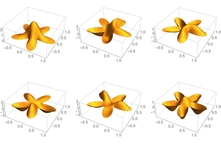
For example, we can draw the first 6 eigenfunction like this:

GraphicsGrid[
 Partition[
  Table[
   eigenvec = ConstantArray[0, Dimensions[stiffness][[2]]]; 
   eigenvec[[intplist]] = Flatten[U[[i]]];
   eigenfun = ElementMeshInterpolation[{Rdiscr}, eigenvec];
   Plot3D[eigenfun[x, y], {x, y} ∈ R],
   {i, 1, 6}], 3],
 ImageSize -> Large]

For the hidden operator L as defined in the comment below, we can easily optain its $L^2$-Moore-Penrose pseudoinverse Lpinv by

(*L=mass2.Transpose[Λ^s U].(U.mass2);*)
Lpinv = b \[Function] Transpose[U].(Λ^-s (U.b));

Next, we solve the reduced equations and write the result into the interior degrees of freedom of a zero vector. Finally, ElementMeshInterpolation provides us with an InterpolatingFunction that can be easily plotted.

solution = ConstantArray[0, Dimensions[stiffness][[2]]];
solution[[intplist]] = Flatten[Lpinv[load2]]; // AbsoluteTiming
solfun = ElementMeshInterpolation[{Rdiscr}, solution];
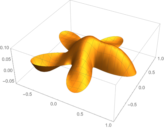
Plot3D[solfun[x, y], {x, y} ∈ R]

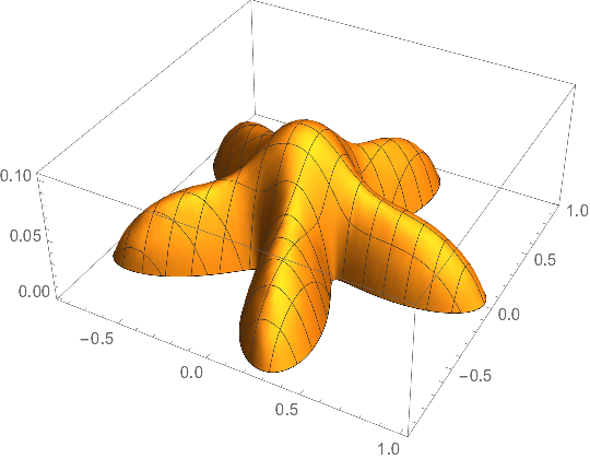
As plausibility check: This is the result for $(-\Delta)^s u = 1$ (upon revisiting this post, I was puzzled by the solution being assymetric while OP asked for the solution of $(-\Delta)^s u = 1$ which ought to have the same symmetries as the domain):

Discussion

This method is however very slow: It has complexity $O(N^3)$, where $N$ is the number of interior vertices. Moreover, this method is not very accurate.

Kernel based methods (e.g., convolution with fundamental solution) might be more accurate and might have complexity $O(N^2)$, but they might be limited to special domains where the fundamental solutions are known.

Speaking about special domains: For the disk $B(0;1) \subset \mathbb{R}^2$, the surface of the sphere $S^2 \subset \mathbb{R}^3$, the unit ball $B(0;1) \subset \mathbb{R}^3$, the standard tori $\mathbb{T}^n = (S^1)^n$, and all cube-like domains like $Q = \coprod_{i=1}^n [a_i,b_i]$, the eigenvectors and eigenvalues are well studied. E.g., using FFT will speed up the process tremendously for $\mathbb{T}^n$ and $Q$.

One could also circumvent the spectral decomposition step by directly assembling the Gagliardo bilinear form $$(u,v) \mapsto \pi^{-(2 s + n/2)}\frac{\Gamma(n/2+s)}{\Gamma(-s)}\int_\varOmega\int_\varOmega \frac{(u(x)-u(y))\,(v(x)-v(y))}{| x-y |^{n + 2 s}}\, \operatorname{d}x \, \operatorname{d}y$$ instead of the Laplacian stiffness matrix ($n=2$) (I am not exactly sure about the multiplicative constant in this formula; I got it from Hitchhiker's Guide to Fractional Sobolev Spaces, p. 8). This would require (partially singular) double integrals over $O(N^2)$ pairs of triangle elements. Moreover, that matrix is dense and needs $O(N^3)$ for factorization. Maybe one can apply FFT on a bounding box of the domain in order to construct a reasonable preconditioner for the conjugate gradient method.