Unexpected behavior of `Exclusions` in `ParametricPlot`

Question

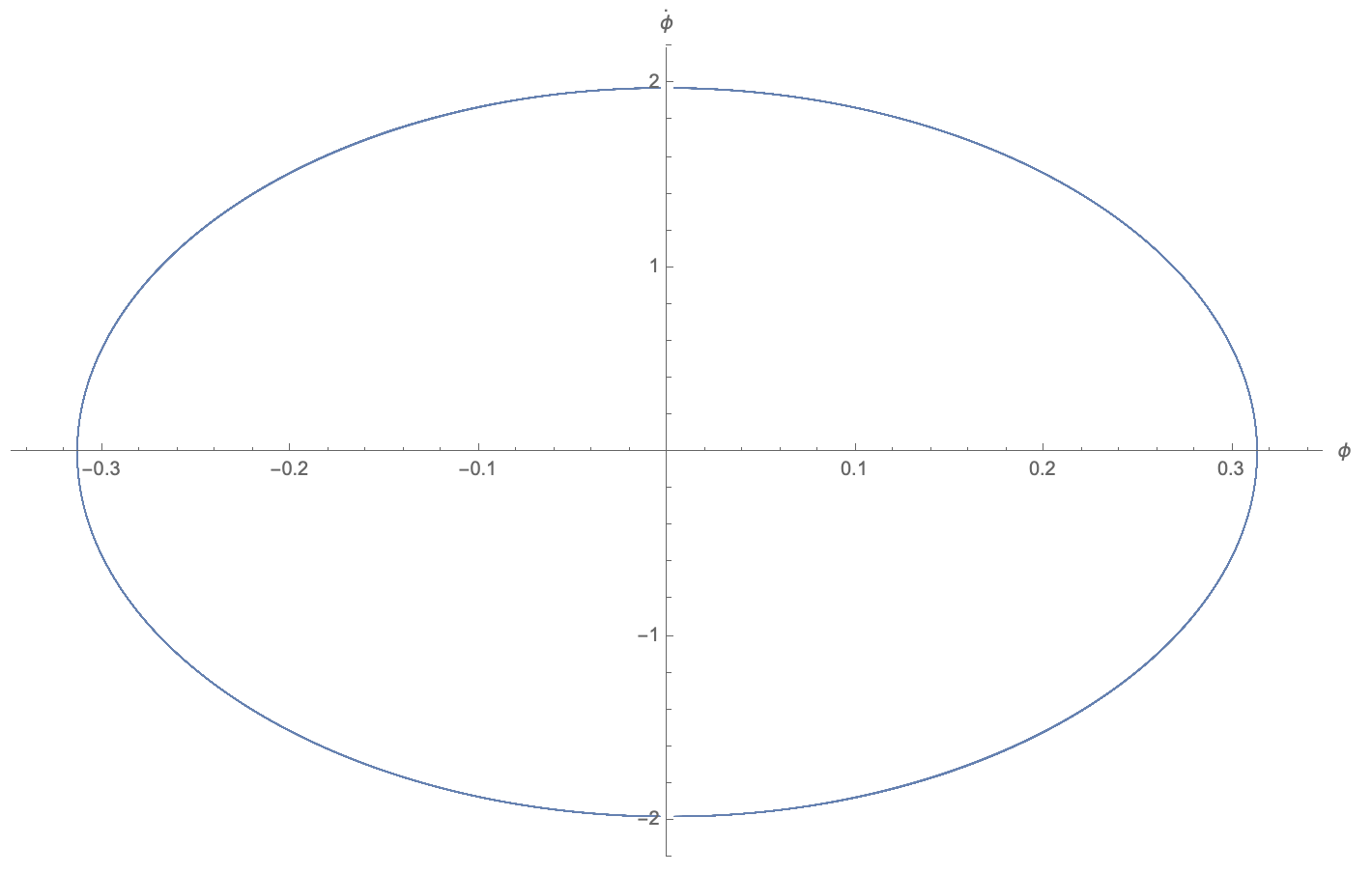
I'm using Mathematica to prepare some teaching materials based on the discussion of the damped, driven pendulum in Chapter 12 of Taylor's Classical Mechanics. This involves using NDSolveValue to solve the non-linear ODE $$ \ddot{\phi} + 2 \beta \dot{\phi} + \omega_0^2 \sin \phi = \gamma \omega_0^2 \cos \omega t. $$ We then want to create a phase plot, which is a parametric curve of the form $(\phi(t), \phi'(t))$ as a function of $t$. This is easy enough to implement:

DDPeq = D[ϕ[t], {t, 2}] + 2 β D[ϕ[t], t] + Subscript[ω, 0]^2 Sin[ϕ[t]] ==
         γ Subscript[ω, 0]^2 Cos[ω t]
paramvals = {ω -> 2 π, Subscript[ω, 0] -> 3 π, β -> 3 π/8, γ -> 1.5}
tmin = 0;
tmax = 200;
ϕsol1[t_] = NDSolveValue[{DDPeq /. paramvals, ϕ[0] == -π/2, ϕ'[0] == 0},
                         ϕ[t], {t, tmin, tmax}];
ParametricPlot[{ϕsol1[t], ϕsol1'[t]}, {t, 0, tmax/4},
  AspectRatio -> 1/GoldenRatio, AxesLabel -> {ϕ, OverDot[ϕ]},
  ImageSize -> Full, PlotPoints -> 100]

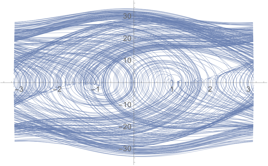
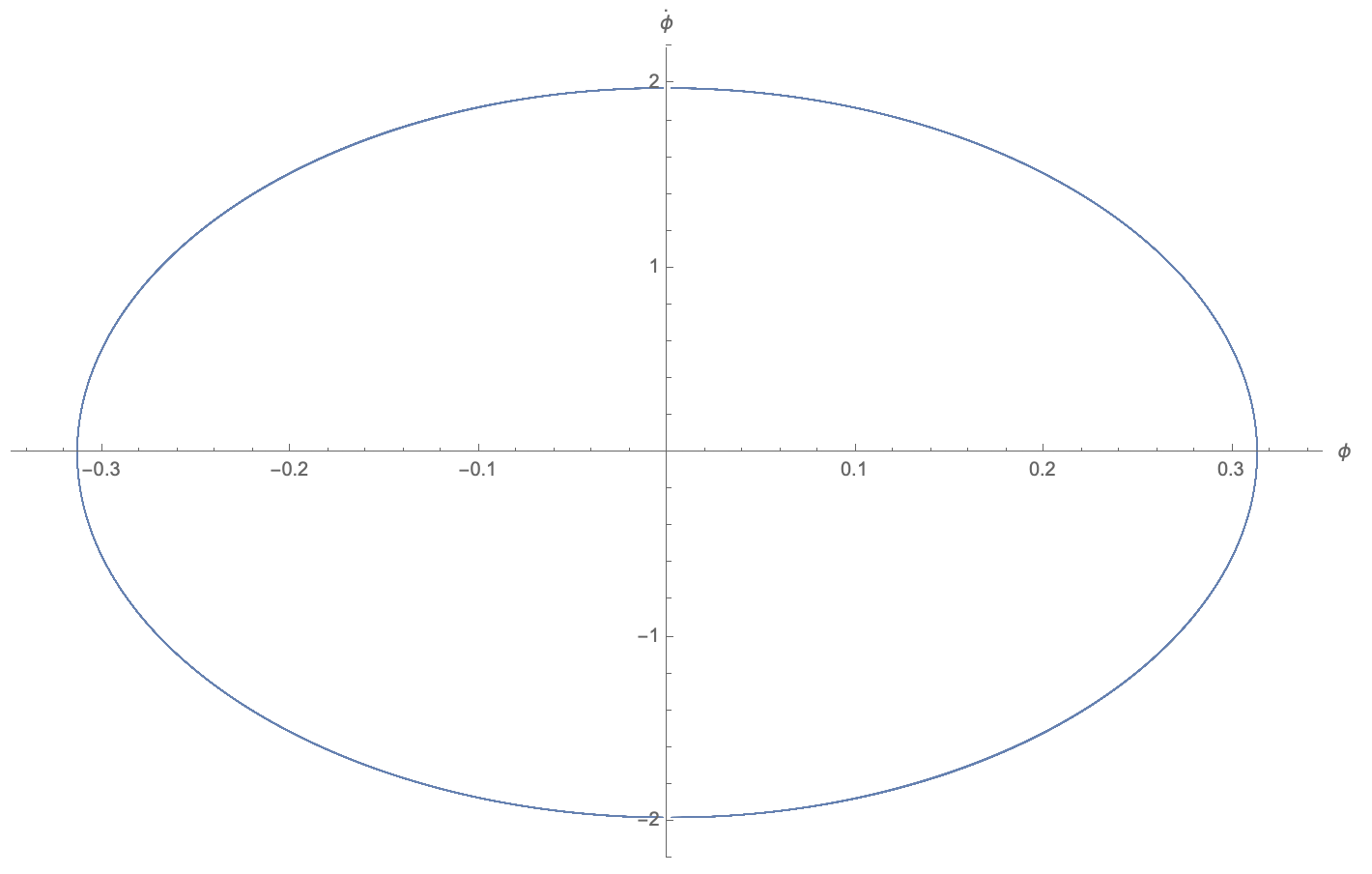
However, the angle of the pendulum is really only defined modulo $2 \pi$; ideally, what we'd like to do is have Mathematica plot with the horizontal axis "wrapped around". We can use Mod to calculate this, and we can use Exclusions to ensure that the opposite edges of the graph aren't connected.

ParametricPlot[{Mod[ϕsol1[t], 2 π, -π], ϕsol1'[t]}, {t, tmax/10, tmax},
  AspectRatio -> 1/GoldenRatio, AxesLabel -> {ϕ, OverDot[ϕ]}, ImageSize -> Full,
  PlotPoints -> 100, Exclusions -> Mod[ϕsol1[t], 2 π] == π, PlotStyle -> Thin]

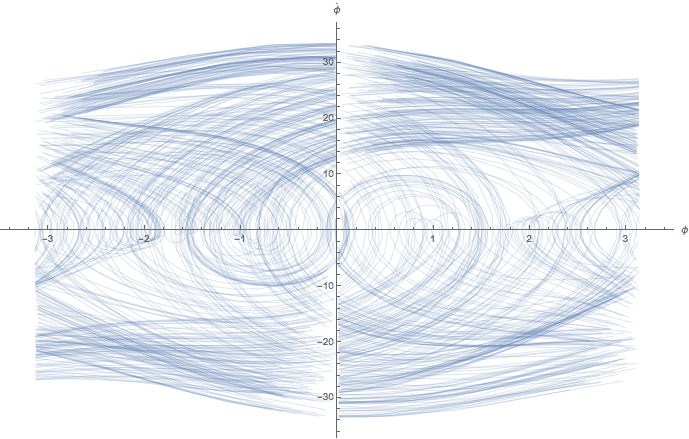
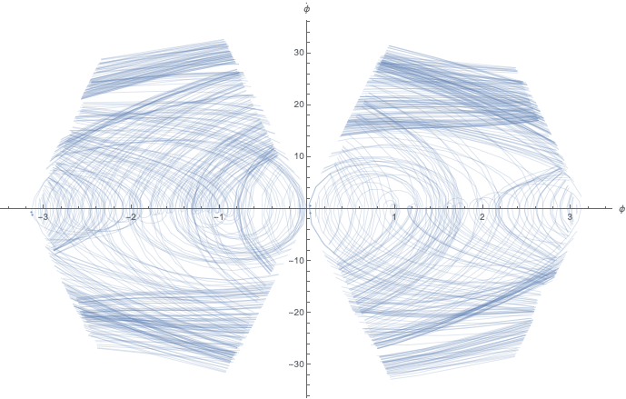
The problem: Mathematica also seems to be "breaking" the plots when $\phi = 0$ (modulo $2 \pi$); you can see that the lines are broken whenever the curve crosses the vertical axis. Increasing PlotPoints makes this problem less noticeable, by narrowing the span of the curve that is omitted (at the edges as well as at the vertical axis); however, the gaps are still present.

Why is Mathematica excluding points that I didn't want it to exclude? Also, is there a better way to create this plot? (I'm still using Mathematica 10.4.1, though my college now has a site license for 11, so if there's a nifty feature in 11 that fixes this problem, I'm all ears.)

---

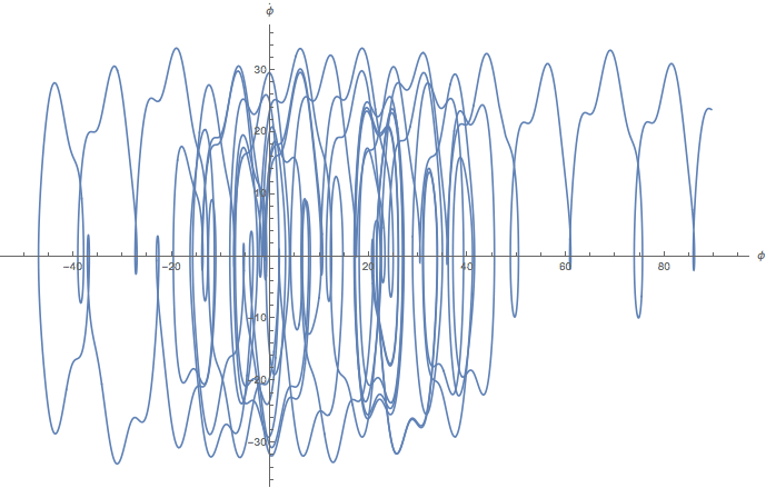
EDIT: Two years later, I'm teaching the course again, and the problem is still bugging me. What's more, the default behavior in Mathematica 12.0 is even worse.

The missing "wedges" get smaller when I increase PlotPoints, but I have to crank that value up to 2000 or so to get a result I find acceptable.

Answer 1

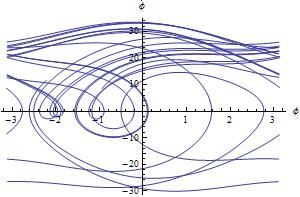
You don't need Exclusion at all. Plot of Mod shows it.

Plot[ Mod[t, 2 π, -Pi], {t, 20, 30}]

ParametricPlot[{Mod[ϕsol1[t], 2 π, -π],  ϕsol1'[
t]}, {t, 20, 30}, AspectRatio -> 1/GoldenRatio,  
AxesLabel -> {ϕ, 
\!\(\*OverscriptBox[\(ϕ\), \(.\)]\)}, ImageSize -> 300,  
PlotPoints -> 100, PlotStyle -> Thin]

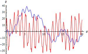
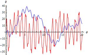
But i think, there is also a problem with accuracy. Compare standart and high precision NDSolve (Since i'm working with Version 8.0, used NDSolve instead of NDSolveValue).

You can not trust result for t > about 10.

ϕsol1 = ϕ /. 
First@NDSolve[{DDPeq /. 
  paramvals, ϕ[0] == -π/2, ϕ'[0] == 0}, ϕ, {t, 
 tmax/10, tmax}, MaxSteps -> 10^5]

ϕsol1a = ϕ /. 
First@NDSolve[{DDPeq /. 
  paramvals, ϕ[0] == -π/2, ϕ'[0] == 0}, ϕ, {t, 
 0, 20}, MaxSteps -> 10^6, WorkingPrecision -> 55, 
AccuracyGoal -> 25, PrecisionGoal -> 25, MaxStepSize -> 10^-3]

Plot[{ϕsol1[t], ϕsol1'[t]}, {t, 0, 20}, 
 AspectRatio -> 1/GoldenRatio, AxesLabel -> {ϕ, 
 \!\(\*OverscriptBox[\(ϕ\), \(.\)]\)}, ImageSize -> 300, 
 PlotPoints -> 100, PlotStyle -> {Blue, Red}]

Plot[{ϕsol1a[t], ϕsol1a'[t]}, {t, 0, 20}, 
  AspectRatio -> 1/GoldenRatio, AxesLabel -> {ϕ, 
\!\(\*OverscriptBox[\(ϕ\), \(.\)]\)}, ImageSize -> 300, 
PlotPoints -> 100, PlotStyle -> {Blue, Red}]

Answer 2

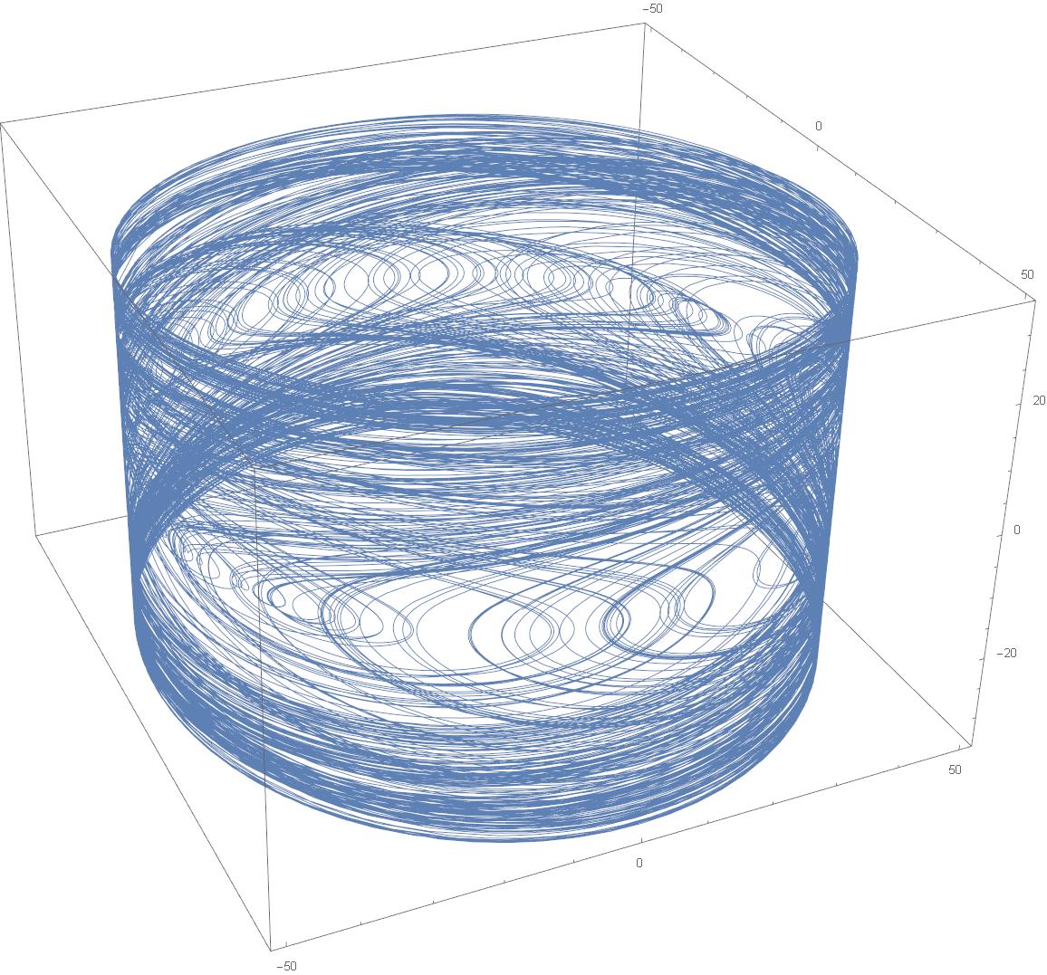
Why not plot the phase space with the true topology?

ParametricPlot3D[{50 Cos[ϕsol1[t]], 50 Sin[ϕsol1[t]], ϕsol1'[t]}, {t, tmax/10, tmax},
                 PlotPoints -> 1000, PlotStyle -> Thin]

Answer 3

As @Akku14 notes, Mod automatically triggers an Exclusion, so no need to add it manually.

Maybe cranking up PlotPoints or MaxRecursion is just your best bet. I find this acceptable and it takes 12 seconds:

ParametricPlot[{Mod[ϕsol1[t], 2 π, -π], ϕsol1'[t]}, {t, tmax/10, tmax},
  AspectRatio -> 1/GoldenRatio, PlotStyle -> Thin, MaxRecursion -> 12]

At least that's the only thing I can come up with!

I guess the wedges appear because ϕ is changing more rapidly when ϕ' is large, so a fixed time buffer around the exclusions translates into a larger gap.

Answer 4

The direct way is simply to increase the number of plot points drastically.

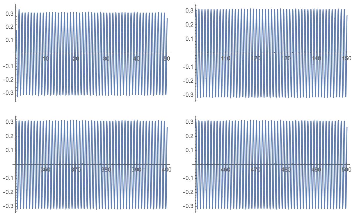
xp = With[{γ = 1/5, ω = 2 π}, 
  Block[{ω0 = 3 ω/2, β}, β = ω0/4;
   x /. First@
     NDSolve[{x''[t] + 
         2 β x'[t] + ω0^2 Sin[
           x[t]] == γ ω0^2 Cos[ω t], 
       x[0] == x'[0] == 0}, x, {t, 0, 500}, MaxSteps -> 1*^5, 
      Method -> "StiffnessSwitching", PrecisionGoal -> 20]]]

{{Plot[xp[t], {t, 0, 50}], 
   Plot[xp[t], {t, 100, 150}]}, {Plot[xp[t], {t, 350, 400}], 
   Plot[xp[t], {t, 450, 500}]}} // GraphicsGrid

With PlotPoints->100 I get the jumps too. With PlotPoints->1500 these are almost gone in phase space (Poisson plot):

ParametricPlot[{Mod[xp[t], 2 π, -π], xp'[t]}, {t, tmax/10, 
  tmax}, AspectRatio -> 1/GoldenRatio,  AxesLabel -> {ϕ, 
\!\(\*OverscriptBox[\(ϕ\), \(.\)]\)}, ImageSize -> Full,  
   PlotPoints -> 1500, Exclusions -> Mod[xp[t], 2 π] == π, 
 PlotStyle -> Thin]

Time can be saved in this case with

ParametricPlot[{Mod[xp[t], 2 π, -π], xp'[t]}, {t, tmax/10, 
  tmax}, AspectRatio -> 1/GoldenRatio,  AxesLabel -> {ϕ, 
\!\(\*OverscriptBox[\(ϕ\), \(.\)]\)}, ImageSize -> Full,  
   PlotPoints -> {150, 2500}, 
 Exclusions -> Mod[xp[t], 2 π] == π, PlotStyle -> Thin]

This example show a technic to work with a mesh and thereupon with mesh refinement: Choosing FEM element type and mesh refinement. It takes more time to work that out. Better improve with the exact solution in this case or the increase in plot points along the y-direction.

The reason for the sparse density of points is that the combination of low phi and high phi' is were rarely taken. At low phi is the driven damped pendulum in downward direction beneath the hold and high phi' means, the pendulum goes there very fast. This fast transit makes intuitively less point in the Poisson phase space plot.

To manage the situation use

AbsoluteOptions.

If the exact solution is in use the inverse can be used to refine the plot point grid at the points under demand.

The SciDraw package is a convenient tool for better plotting with Mathematica. It is free and makes refinement of plot points in parts of a plot accessible.

Another idea is to use ScalingFunctions. It can plot with the inverse function f^-1. An example is plotting with a user-defined scaling function or nicer How to use Scaled function [closed]

Or make use of Piecewise.

To reduce number of plot points use the symmetry argument.

This is another question for the forced damped oscillator. It provides ideas about how to stick to more precise trajectories.

This is a fully fledged working example Forced Oscillator with Damping and there are many more.