Resonance Curve using NDSolve

Question

I am trying to make a resonance curve like this one below, using NDSolve.

I tried to use code as below. Basically I try to hold solution for a w (driving frequency value) using NumericQ and then find the max amplitude using FindMaxValue when t is big enough. But my code returns a lot of error code I don't understand. By the way, I am using NDSolve directly, so I can test the accurateness of NDSolve Method.

ClearAll;

f[w_?NumericQ] := 
Block[{sol}, 
  sol = NDSolve[{x''[t] + x'[t] + x[t] == Cos[w*t], x[0] == 0, x'[0] == 0}, 
    x[t], {t, 0, 100}];
 (FindMaxValue[x[t], {t, 50}])[[1]]]

ListLinePlot[Table[f[w], {w, 0, 100, 1}], DataRange -> {0, 100}]

Answer 1

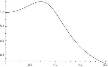
Given the nature of a forced, damped oscillator, an efficient way to approximate the resonance curve is to use WhenEvent (or EventLocator) to locate a maximum after the transient solution effectively vanishes.

Clear[amp];
amp[w_] /; w == 0 = 1.;
amp[w_?NumericQ] :=
 Block[{x},
  #[#["Domain"][[1, -1]]] &[
   x /. First@NDSolve[{
       x''[t] + x'[t] + x[t] == Cos[w*t], x[0] == 0, x'[0] == 0, 
       WhenEvent[x'[t] < 0 && t > 100, "StopIntegration"]}, 
      x, {t, 0, 100 + 3 Pi/w}]
   ]
  ];

Plot[amp[w], {w, 0, 2}]

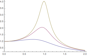
We can extend it to a more general DE:

amp[w_, w0_?NumericQ, damping_?NumericQ] /; w == 0 = 1.;
amp[w_?NumericQ, w0_?NumericQ, damping_?NumericQ] :=
 Block[{x},
  #[#["Domain"][[1, -1]]] &[
   x /. First@NDSolve[{
       x''[t] + 2 damping w0 x'[t] + w0^2 x[t] == Cos[w*t],
       x[0] == 0, x'[0] == 0, 
       WhenEvent[x'[t] < 0 && t > 40/damping, "StopIntegration"]}, 
      x, {t, 0, 50/damping + 3 Pi/w}]
   ]
  ];

Plot[Evaluate[Table[amp[w, 1, z], {z, {1/2, 1/4, 1/8}}]], {w, 0, 2}]

---

On the # and "Domain"

The # is a Slot. It represents the (first) argument of a Function usually constructed with a & (often called a "pure function"). The argument is the solution x /. First@NDSolve[..], which is an InterpolatingFunction.

The #[#["Domain"][[1, -1]]] &[ifn] evaluates an InterpolatingFunction solution ifn at the end point of its domain (explained below). In this case, the end point is the point at which the integration stopped, and it yields the maximum value of the solution to the differential equation. (Technically, it is a local maximum, which approximates the amplitude of the steady-state solution.) An InterpolatingFunction might look something like this in a notebook:

ifn = x /. First@NDSolve[{
     x''[t] + x'[t] + x[t] == Cos[1.3 t], x[0] == 0, x'[0] == 0, 
     WhenEvent[x'[t] < 0 && t > 80, "StopIntegration"]}, 
    x, {t, 0, 100 + 3 Pi}]

(* InterpolatingFunction[{{0., 83.7484}}, <>] *)

Note that the domain is displayed. Others have wondered what properties are inside ifn here: What's inside InterpolatingFunction[{{1., 4.}}, <>]? There are methods for accessing these properties through the "DifferentialEquations`InterpolatingFunctionAnatomy`" package, described in tutorial/NDSolvePackages. There are some shortcuts to these methods. If ifn is an InterpolatingFunction, then the following lists them:

ifn["Methods"]

(* {"Coordinates", "DerivativeOrder", "Domain", "ElementMesh", 
    "Evaluate", "Grid", "InterpolationOrder", "MethodInformation", 
    "Methods", "Periodicity", "Properties", "QuantityUnits", 
    "ValuesOnGrid"} *)

They may be invoked by ifn[method]:

ifn["Domain"]
(* {{0., 83.7484}} *)

The point at which the maximum occurs is the end point of the domain, given by

ifn["Domain"][[1, -1]]
(* 83.7484 *)

To summarize, #[#["Domain"][[1, -1]]] &[x /. First@NDSolve[..]] is short for

ifn = x /. First@NDSolve[..];
ifn[ifn["Domain"][[1, -1]]]

which may be broken down further as

ifn = x /. First@NDSolve[..];
domains = ifn["Domain"];  (* domains of each independent variable *)
tdomain = First[domains]; (* the first domain *)
tfinal = Last[tdomain];   (* right end point of domain *)
ifn[tfinal]

A note on the NDSolve parameters

The amplitude of the transient solution decays as Exp[-damping t]. The 40/damping was chosen so that the amplitude would be extremely small, less than 10.^-16, or equivalently, so that t > 36.8414/damping. It was rounded up to 40. A slight gain in speed may be obtained by increasing this tolerance. (For example, plotting was about 15-25% faster if the integration stops when t > 20/damping and the transient amplitude is less than 10^-8.)

The interval of integration {t, 0, 50/damping + 3 Pi/w} has to extend at least one period beyond 40 / damping when we start looking for a maximum. The time 50/damping + 3 Pi/w should be sufficiently large since 50/damping > 40/damping and 3 Pi/w > 2 Pi/w. Since the integration stops before this, it doesn't really matter if a little extra is thrown in.