Representative Smooth Kernel Distribution from Truncated Distribution

Question

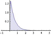
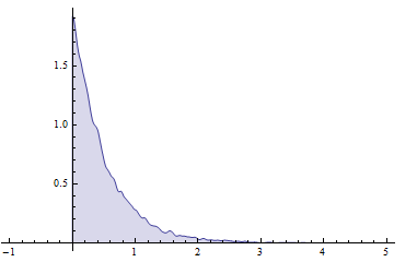
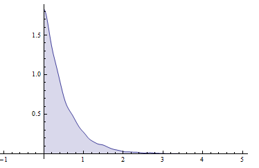
I am trying to produce a better distribution from a dataset that is bounded to be greater than 0. Here is an example distribution from the documentation that mimics the behavior of the actual dataset:

data = RandomVariate[ExponentialDistribution[2], 10^4];
dist = SmoothKernelDistribution[data];
\[ScriptCapitalD] = TruncatedDistribution[{0, Infinity}, dist];
Plot[Evaluate@PDF[\[ScriptCapitalD], x], {x, -1, 5}, PlotRange -> All,
  Filling -> Axis]

As you can see, the peak of the SmoothKernelDistribution is not at 0, but at some value slightly greater than zero. The more points there are in the dataset, the closer the peak is to zero, as there will be a point in the dataset that is closer and closer to zero with more points. In the real dataset, I don't have the liberty of drawing more points, but I do know that the real dataset is restricted to be > 0.

Using the standard histogram, the peak will be 0 given a large enough bin size, which I guess can be achieved in SmoothKernelDistribution by increasing the kernel width, but as far as I can tell SmoothKernelDistribution does not automatically set this width to avoid the above behavior. My question is: How do I generate a SmoothKernelDistribution which mimics the behavior of the underlying distribution?

Answer 1

As of version 9 there is an undocumented extension to the kernel functions which allows you to bound the domain. You do this by specifying the kernel function as {"Bounded", c, ker} where c is the left boundary (0 in your case) and ker is the usual kernel function. You can also allow for both the left and right to be bounded via {"Bounded", {c1, c2}, ker}. Bounding only on the right can be done using c1 = -Infinity.

This works by reflecting part of the data about the boundaries and subsequently truncating the resulting estimate. As this is undocumented I make no promises that it won't someday change or that it is 100% tested.

data = RandomVariate[ExponentialDistribution[2], 10^4];
dist = SmoothKernelDistribution[data, Automatic, {"Bounded", 0, "Gaussian"}];
Plot[Evaluate@PDF[dist, x], {x, -1, 5}, PlotRange -> All,Filling -> Axis]

Edit:

To do something similar without M9 (though not in full generality) you can try reflecting the data about the y-axis and truncate yourself.

data = RandomVariate[ExponentialDistribution[2], 10^4];
pseudodata = Join[-data, data];
dist = TruncatedDistribution[{0, \[Infinity]}, 
   SmoothKernelDistribution[pseudodata]];
Plot[PDF[dist, x], {x, -1, 5}, PlotRange -> All, Filling -> Axis]