Here is a possible solution.
Given a cut point c we can create a kernel density estimate kde truncated on {-Infinity, c} and a tail estimate tail truncated on {c, Infinity} with the additional restriction that the PDF of the tail at c must be equal to PDF[kde, c].
To solve for this point in a way that is robust enough for a variety of data sets and distributions we need to set up special rules for dealing with likelihoods.
The function bound will be used to ensure that indeterminate values of the LogLikelihood for our restricted tail will allow optimization functions to keep searching.
bound[Infinity] := $MinMachineNumber
bound[-Infinity] := $MinMachineNumber
bound[n_?NumericQ] := n
Now for the tail estimator. The 1000 $MachineEpsilon is to nudge us away from restricted boundaries (and may need adjusted). The initial call to FindDistributionParameters attempts to get good starting values.
tailEstimate[dist_, data_, prob_, c_] :=
 Block[{params, est, tdist},
  params = FindDistributionParameters[data, dist];
  tdist = TruncatedDistribution[{c, \[Infinity]}, dist];
  est = Apply[
    FindMaximum, {{bound[
       LogLikelihood[tdist, Cases[data, x_ /; x > c]]],
      DistributionParameterAssumptions[tdist] &&
       PDF[tdist, c + 1000 $MachineEpsilon] == prob},
     params /. Rule -> List}];
  tdist /. est[[2]]
  ]
Now to put it together with the kernel density estimator.
kde[data_, bw_, c_, tailModel_] :=
 Block[{kern, tail},
  kern = TruncatedDistribution[{-\[Infinity], c}, KernelMixtureDistribution[data, bw]];
  tail = tailEstimate[tailModel, data, PDF[kern, c], c];
  MixtureDistribution[{1, 1}, {kern, tail}]
  ]
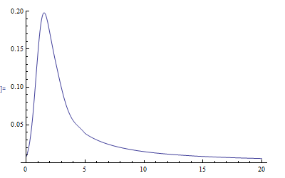
Here is an example using heavy tailed data.
data = RandomVariate[ParetoDistribution[1, .5], 1000];
mdist = kde[data, .5, 5, ParetoDistribution[a, b]];
Plot[PDF[mdist, t], {t, 0, 20}, PlotRange -> {0, .2}]


 Thank you!

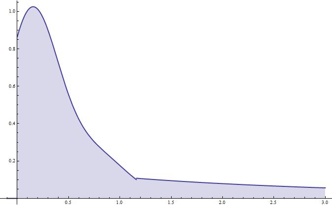
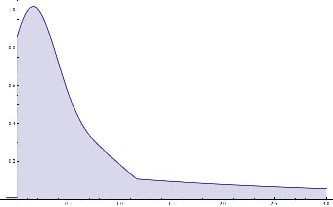
SmoothKernelDistributionon your data and how you "paste them together". If you do this incorrectly you'll end up with a distribution that doesn't add up to a probability of 1. Could you provide a small example? $\endgroup$SmoothKernelDistributionthat I reported, see the discussion after @rm -rf's answer to How to create a heatmap from list of coordinates? $\endgroup$