The definition of the distribution is actually give in the documentation, and it should be rather straight forward to port it. The definition is
$$
f(x) = \frac{1}{n h}\sum^n_{i=1}k\left(\frac{x-x_i}{h}\right).
$$
The only unknown here is h, the bandwidth, which can be extracted from the DataDistribution object.
Sample distribution and data:
dist = MixtureDistribution[
   {1, 2},
   {NormalDistribution[], NormalDistribution[2, 1/2]}
   ];

data = RandomVariate[dist, 10^4];
dataDist = SmoothKernelDistribution[data];
Now we can extract values as follows:
sampleY = dataDist[[2, 1]];
sampleX = dataDist[[2, 2]];
bandwidth = dataDist[[2, 3]];
Using the bandwidth, we can now compute the probability density for an arbitrary x, in a way that's easy to port to other languages because it only requires basic math functions. I'm going to use a Gaussian kernel, which is the default (look in the documentation for the definition of other kernels):
k[u_] := (1./Sqrt[2. Pi]) Exp[-u^2./2.]
f[x_, h_] := (1/(Length[data] h)) Sum[k[(x - xi)/h], {xi, data}]
To see that f[x_, h_] works, we can compute it for the sample points given in the DataDistribution object:
samplePts = {#, f[#, bandwidth]} & /@ sampleX;
Plot[
 PDF[dataDist, x], {x, -4, 4},
 Epilog -> {
   Red,
   PointSize[Small],
   Point@samplePts
   }]

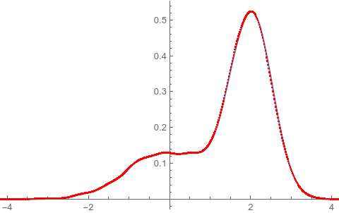
This picture shows that the formula works, and returns the same values as PDF[dataDist, x] does. As pointed out in the comments, Mathematica applies some interpolation. I don't think you need to bother to port the exact interpolation method to your other language, it doesn't look like it would make any difference. And in any case, you have the formula so you can compute the PDF with arbitrary precision.


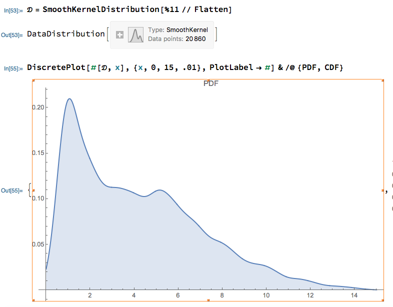
PDF[\[ScriptCapitalD], x], you'll see that the functional form is a Hermite interpolation function, which would be rather tedious to port over. You might have more luck withKernelMixtureDistribution, which returns a sum of Gaussians. $\endgroup$