Finding a best fit without having to specify the form of the equation

Question

Well the title actually says it all. Is there a function that finds the best fit for data points without any user-inputed information about the form the formula might have?

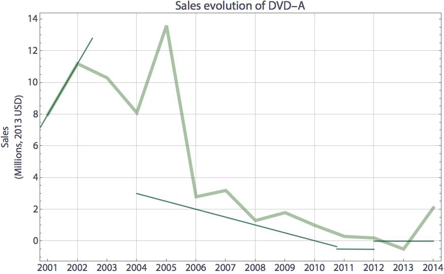
Here is the data I want to find a fit for: data={8, 11.2, 10.3, 8.1, 13.6, 2.8, 3.2, 1.3, 1.8, 1, 0.3, 0.2, 0, 2.1} It is the annual sales of DVD-A from 2001 to 2014 (this is the whole dataset). In 2003, a direct competitor to the DVD-A appeared, the SA-CD. So I would like to graphically illustrate the fact that the trend in the sales of the DVD-A change drastically from the moment the SA-CD made it's appearance. Obviously, there are only two observations before 2003, so a linear fit is obvious... But I'm having trouble finding a continuous function that illustrates the sales trend from 2003 to 2014.

So the predictor variable is simply {3,4,...,14}.

Here is a graph of the data, the linear trend for the years 2001 and 2002 and the chopped-up function for the 2003-2014 period provided by the FindFormula described below:

Code for the graph:

Show[ListLinePlot[data,(*DVD-A*) PlotStyle ->Directive[CMYKColor[0.37,0.,0.44,0.48] ,Thickness[.008],Opacity[.5]] ,Frame -> True ,PlotRange -> All ,FrameTicks-> {Automatic, {Table[{i, 2000 + i}, {i, 0, 14}], None}} ,PlotLabel -> "Sales evolution of DVD-A" ,FrameLabel -> {None, "Sales\n(Millions, 2013 USD)"}] ,Plot[Evaluate@LinearModelFit[data[[{1,2}]], t, t][t], {t, 0.75, 2.5}] ,Plot[Evaluate@FindFormula[data[[3;;]], t, 5,SpecificityGoal -> 3][[4]], {t,4, 14}] ]

Until now, I have tried this: FindFormula[data[[3;;]], t, 5, SpecificityGoal -> 3], which gives a chopped-up fonction with different chunks. I would like to find a continuous function that fits the data (I already tried with NonlinearFit with different orders polynomials and did not get a visually good estimation of the data from 2003 to 2014).

Thanks,

Answer 1

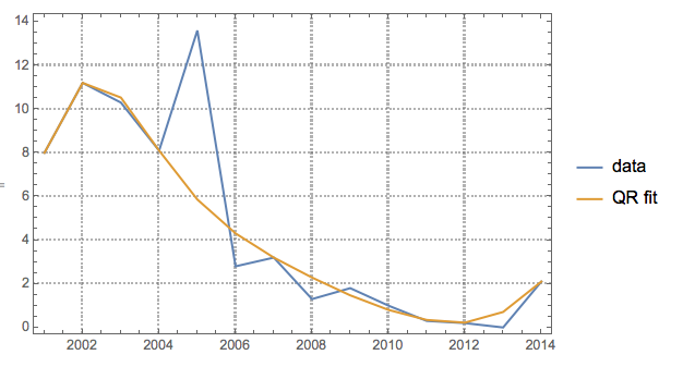
Using Quantile regression might produce results you would want.

Import["https://raw.githubusercontent.com/antononcube/MathematicaForPrediction/master/QuantileRegression.m"]

data = {8, 11.2, 10.3, 8.1, 13.6, 2.8, 3.2, 1.3, 1.8, 1, 0.3, 0.2, 0, 2.1};
ts = Transpose[{Range[2001, 2014], data}];

qfunc = QuantileRegression[ts, 4, {0.5}][[1]];

ListLinePlot[{ts, {#, qfunc[#]} & /@ ts[[All, 1]]}, 
 PlotLegends -> {"data", "QR fit"}, PlotTheme -> "Detailed"]

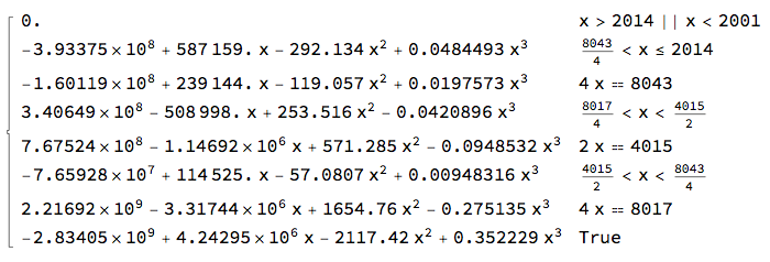
qfunc[x] // Simplify

Answer 2

I think that @m_goldberg had the right answer in his comment: "I don't think there is any answer to this question..."

Why do I say this? Mainly because of the subjective tone you've used. In other words, when a good curve appears, you'll know it when you see it. That is not to say that such an approach is wrong. It's only to say that maybe the rest of us can't help you because of that.

In addition, there are some statements for which there is not much statistical validity:

(1) "Obviously, there are only two observations before 2003, so a linear fit is obvious..." No, it not obvious but it is inappropriate.

(2) Both DVD-A and SA-CD have had low sales, have never caught on (few musicians recording in such formats), and finding a smooth curve to fit 12 data points won't help you with assigning cause-and-effect. You mention difference-in-difference techniques which are popular among certain disciplines but the restrictive assumptions are rarely checked and maybe rarely met.

(3) You've given a good rationale for why the sales are negative in one year (because of returns) but no rationale for why converting that to a zero would be appropriate as other years have returns also.

(4) FindFormula does not give "a chopped-up fonction with different chunks". It gives you the top 5 models that you requested.

I'd still recommend first addressing the question at CrossValidated and then using Mathematica for implementation.

Update: Why you need confidence bands

At some point adding in more parameters loses effectiveness in fitting and soon one starts to overfit giving you false confidence in the result. Two ways of assessing the models being considered is to use confidence bands and ranking models by their AICc statistic. (Overfitting especially applies to good but data hungry techniques such as quantile regression and generalized additive models when one doesn't have many data points to estimate the multiple and "hidden" parameters.)

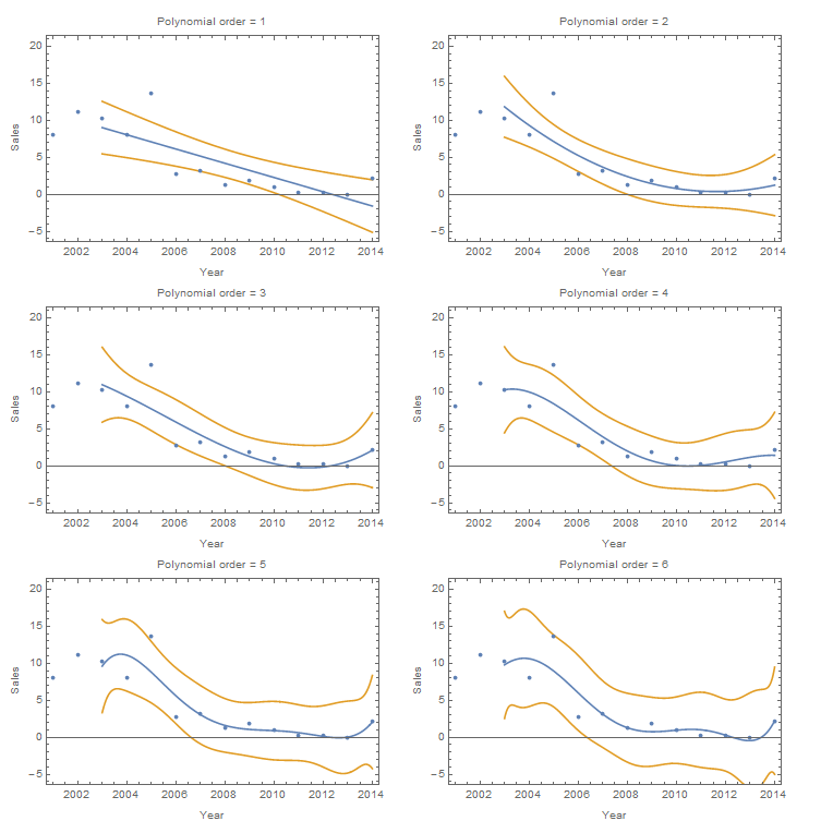
Here is a summary of fits if you restrict yourself to polynomials of order up to 6 for predicting the values for the years 2003 through 2014.

data = {8, 11.2, 10.3, 8.1, 13.6, 2.8, 3.2, 1.3, 1.8, 1, 0.3, 0.2, 0, 2.1};
ts = Transpose[{Range[2001, 2014], data}];
ts2 = Transpose[{Range[3, 14], data[[Range[3, 14]]]}];

fit[order_] := Module[{x, z, i, lm},
  lm = LinearModelFit[ts2, Table[x^i, {i, order}], x];
  Show[Plot[{lm[z - 2000], lm["MeanPredictionBands"] /. x -> z - 2000}, {z, 2003, 2014}],
   ListPlot[ts], AxesOrigin -> {2000, 0}, 
   PlotRange -> {{2001, 2014}, {-5, 20}}, ImageSize -> Medium,
   Frame -> True, 
   FrameLabel -> {{"Sales", ""}, {"Year", 
      "Polynomial order = " <> ToString[order]}}]
  ]

Grid[{{fit[1], fit[2]}, {fit[3], fit[4]}, {fit[5], fit[6]}}]

One can see that as the order of the polynomial increases, there is closer agreement to the observed data. However, a price is paid in that the confidence bands start to get wider and wider.

If one computes the AICc statistic, the 2nd order polynomial has the smallest AICc statistic with the linear model (1st order polynomial) coming in second. So if you restrict yourself to these polynomials the 2nd order polynomial is best. Whether or not the confidence bands are small enough to meet your objective is a subject matter issue. But ignoring the confidence bands is not justifiable.