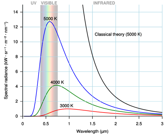
I am trying to extract a curve from a scanned graph and find a best fit equation. For example, starting from:

How could one find an equation starting from the image file ?
I am trying to extract a curve from a scanned graph and find a best fit equation. For example, starting from:

How could one find an equation starting from the image file ?
Here's something to get you started, (assembled from Andy Ross' code). Data points are extracted from a data series in an image.
Your original image will need some editing in order to process each curve separately.
The following tadpoles plot is used for example.
img = Import@"http://www.biologycorner.com/resources/graph_tadpoles.JPG";
data = Round[ImageData[img], 1];
col = DeleteDuplicates[Flatten[Round[ImageData[img], 1], 1]];
Graphics[{RGBColor[#], Disk[]}, ImageSize -> Tiny] & /@ col
Select which colour to extract, col[[3]]:
binImage = Image@Replace[data, {col[[3]] -> 1, _ :> 0}, {2}];
curve = ImageApply[{0, 0, 0} &, binImage,
   Masking -> ColorNegate[Binarize[GaussianFilter[binImage, 5]]]];
curvLoc = (Reverse /@ Position[ImageData[curve, DataReversed -> True], {1., 1., 1.}]);
ListPlot[curvLoc, PlotRange -> All, ImageSize -> 500]
Extract the top line.
groups = GatherBy[curvLoc, First];
maxes = Last@Sort@# & /@ groups;
ListLinePlot[Sort@maxes, ImageSize -> 500]
Note this actually is the top line. You'll have to judge whether adjustment is needed.
Show[ListPlot[curvLoc, PlotRange -> All, PlotStyle -> Directive[Thick, Orange]],
 ListLinePlot[Sort@maxes], ImageSize -> 800]
From there you can analyse the data points.
To scale the data points it's helpful if the original image is clipped to know axis dimensions. Then you can use ImageDimensions to scale the data.
Well, you have two questions in one: (1) How to "take" the curve from the image into Mma? and (2) How to fit it?.
Here I address the first question and give one possible solution aditional to the ones offered before.
Some time ago I published a function copyCurve on this site, along with its detailed description. You can take it from there.
Copy the image from the screen (Right click, and choose "Copy image") and paste it inside the brackets of the function copyCurve
copyCurve[place your image here]
Evaluate the resulting expression.
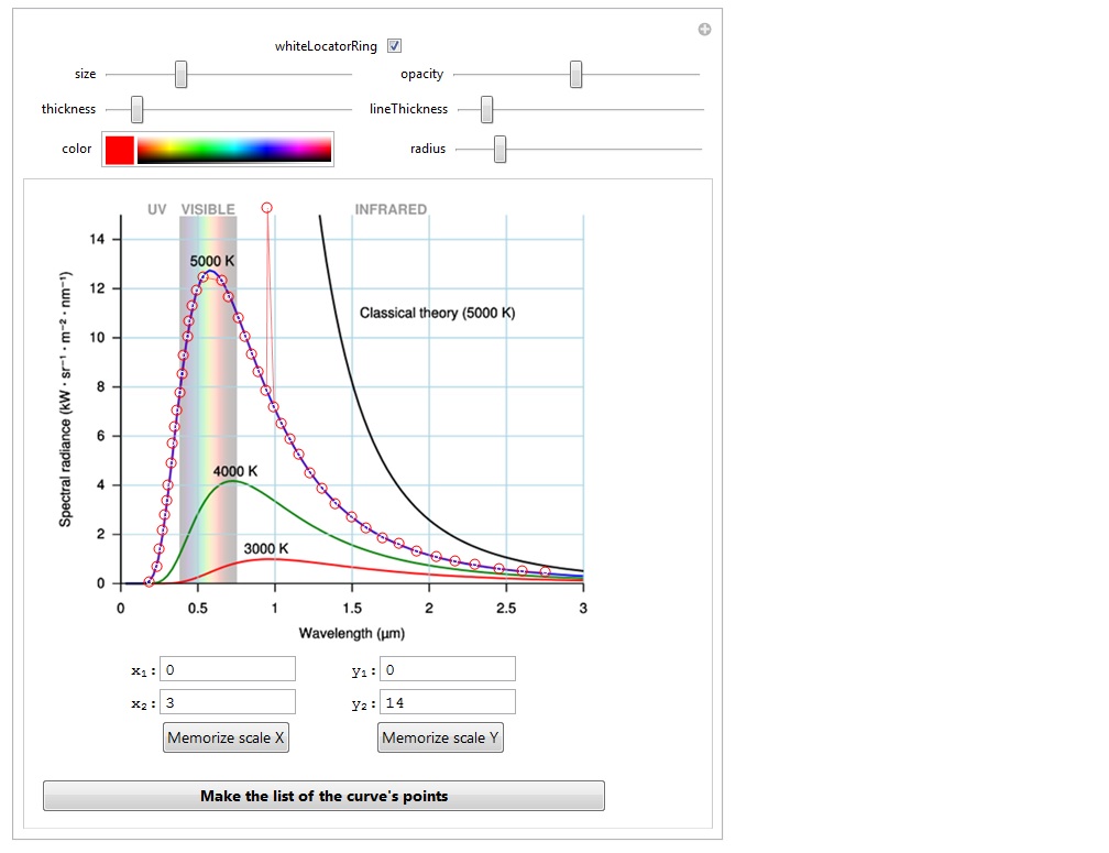
Follow the instructions for the program published on the site mentioned above and place the cursors along the curve of your choice. I have chosen the blue one for the sake of example. You should obtain something like this:

As soon as this is done, press the button "Make the list of the curve points" and then in a separate cell evaluate the variable listOfPoints. You will get the following list for the blue line:
{{0.191, -0.021}, {0.24, 0.645}, {0.261, 1.36}, {0.283, 2.101}, {0.294, 2.742}, {0.31, 3.314}, {0.315, 3.952}, {0.336, 4.862}, {0.347, 5.635}, {0.358, 6.309}, {0.374, 7.015}, {0.39, 7.722}, {0.411, 8.462}, {0.416, 9.236}, {0.443, 10.01}, {0.454, 10.651}, {0.475, 11.256}, {0.502, 11.895}, {0.544, 12.434}, {0.598, 12.635}, {0.662, 12.298}, {0.71, 11.626}, {0.769, 10.784}, {0.817, 10.01}, {0.859, 9.303}, {0.902, 8.564}, {0.95, 7.824}, {0.998, 7.15}, {1.052, 6.442}, {1.105, 5.837}, {1.158, 5.199}, {1.233, 4.458}, {1.313, 3.817}, {1.399, 3.179}, {1.505, 2.64}, {1.596, 2.205}, {1.703, 1.799}, {1.81, 1.56}, {1.922, 1.261}, {2.055, 1.026}, {2.173, 0.857}, {2.301, 0.722}, {2.456, 0.553}, {2.605, 0.453}, {2.76, 0.385}}
Done.
Now you can fit it. To do this you need to have a function to which you are going to fit the data. Since you gave no function, I cannot help you further.
Have fun!
Edit: to address your second question. First of all the Planck if you use the Planck distribution, then the only fitting parameter may be the temperature. So you should not fix it to constant. Second, do not forget that your plot is not given in SI units, while the Planck formula you gave operates with them. So you need to adapt them. You might want to operate as follows:
  Clear[lst];
lst = {{0.191`, -0.021`}, {0.24`, 0.645`}, {0.261`, 1.36`}, {0.283`,
     2.101`}, {0.294`, 2.742`}, {0.31`, 3.314`}, {0.315`,
     3.952`}, {0.336`, 4.862`}, {0.347`, 5.635`}, {0.358`,
     6.309`}, {0.374`, 7.015`}, {0.39`, 7.722`}, {0.411`,
     8.462`}, {0.416`, 9.236`}, {0.443`, 10.01`}, {0.454`,
     10.651`}, {0.475`, 11.256`}, {0.502`, 11.895`}, {0.544`,
     12.434`}, {0.598`, 12.635`}, {0.662`, 12.298`}, {0.71`,
     11.626`}, {0.769`, 10.784`}, {0.817`, 10.01`}, {0.859`,
     9.303`}, {0.902`, 8.564`}, {0.95`, 7.824`}, {0.998`,
     7.15`}, {1.052`, 6.442`}, {1.105`, 5.837`}, {1.158`,
     5.199`}, {1.233`, 4.458`}, {1.313`, 3.817`}, {1.399`,
     3.179`}, {1.505`, 2.64`}, {1.596`, 2.205`}, {1.703`,
     1.799`}, {1.81`, 1.56`}, {1.922`, 1.261`}, {2.055`,
     1.026`}, {2.173`, 0.857`}, {2.301`, 0.722`}, {2.456`,
     0.553`}, {2.605`, 0.453`}, {2.76`, 0.385`}} /. {x_,
     y_} -> {x*10^-6, y*10^12};
model = (2*h*c^2)/\[Lambda]^5*1/(Exp[(h*c)/(\[Lambda]*k*T)] - 1)
ff = FindFit[lst, model, {{T, 4000}}, \[Lambda]]
yielding
(* {T -> 4974.56} *)
Alternatively you may do this:
 Manipulate[
 Show[{

   Plot[(2*h*c^2)/\[Lambda]^5*1/(
     Exp[(h*c)/(\[Lambda]*k*T)] - 1), {\[Lambda], 0, 3*10^-6}],
   ListPlot[lst]

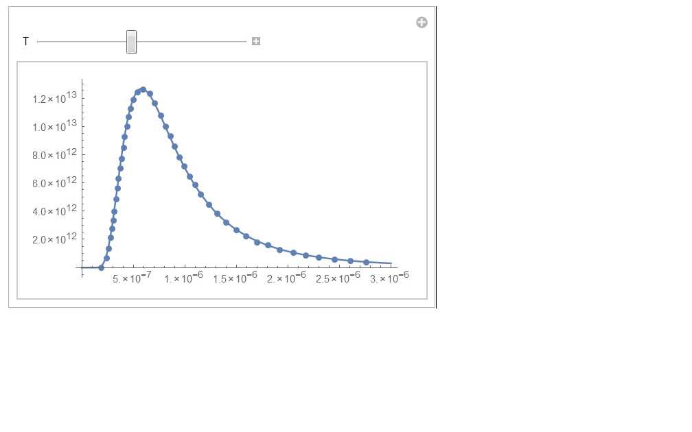
   }], {{T, 4990}, 4900, 5100}]
you should obtain this:

Once more, have fun!
h = 6.6260693*10^-34; c = 2.99792458*10^8; k = 1.3806505*10^-23; tmp = 5000; planckfunction[tmp_, lambda_] := 2 h c^2/(((lambda*10^-6)^5) (Exp[h c/((lambda*10^-6) k tmp)] - 1)); Plot[planckfunction[tmp, lambda], {lambda, 0, 3}]
$\endgroup$
Commented
Nov 7, 2014 at 11:58