Regarding phase space diagram/trajectory

Question

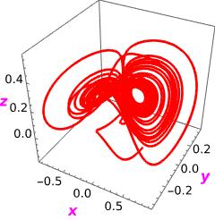
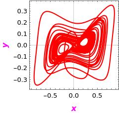
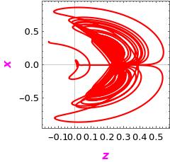
I have a 3D chaotic system and its one 3D phase-space portrait and three 2D phase-space portrait (x-y plane, y-z plane, z-x plane) are given below.

s = NDSolve[{Derivative[1][x][t] == -0.4*x[t] + y[t] + 10.0*y[t]*z[t],
     Derivative[1][y][t] == -x[t] - 0.4*y[t] + 5.0*x[t]*z[t], 
    Derivative[1][z][t] == 0.175*z[t] - 5.0*x[t]*y[t], x[0] == 0.349, 
    y[0] == 0.0, z[0] == -0.160}, {x, y, z}, {t, 0, 600, 0.01}, 
   MaxSteps -> \[Infinity]];
p1 = ParametricPlot3D[Evaluate[{x[t], y[t], z[t]} /. s], {t, 0, 300}, 
  PlotRange -> Full, PlotPoints -> 200, 
  AxesLabel -> {Style[x, Medium, Bold, Magenta], 
    Style[y, Medium, Bold, Magenta], 
    Style[z, Medium, Bold(*Plain*), Magenta]}, 
  LabelStyle -> Directive[Black, Plain], PlotTheme -> "Scientific", 
  PlotStyle -> Red, ImageSize -> Small, BoxRatios -> {1, 1, 1}]
p2 = ParametricPlot[Evaluate[{x[t], y[t]} /. s], {t, 0, 300}, 
  PlotRange -> Full, PlotPoints -> 200, 
  FrameLabel -> {Style[x, Medium, Bold, Magenta], 
    Style[y, Medium, Bold, Magenta]}, 
  LabelStyle -> Directive[Black, Plain], PlotTheme -> "Scientific", 
  PlotStyle -> Red, ImageSize -> Small, AspectRatio -> 1]
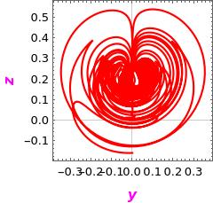
p3 = ParametricPlot[Evaluate[{y[t], z[t]} /. s], {t, 0, 300}, 
  PlotRange -> Full, PlotPoints -> 200, 
  FrameLabel -> {Style[y, Medium, Bold, Magenta], 
    Style[z, Medium, Bold(*Plain*), Magenta]}, 
  LabelStyle -> Directive[Black, Plain], PlotTheme -> "Scientific", 
  PlotStyle -> Red, ImageSize -> Small, AspectRatio -> 1]
p4 = ParametricPlot[Evaluate[{z[t], x[t]} /. s], {t, 0, 300}, 
  PlotRange -> Full, PlotPoints -> 200, 
  FrameLabel -> {Style[z, Medium, Bold, Magenta], 
    Style[x, Medium, Bold(*Plain*), Magenta]}, 
  LabelStyle -> Directive[Black, Plain], PlotTheme -> "Scientific", 
  PlotStyle -> Red, ImageSize -> Small, AspectRatio -> 1]

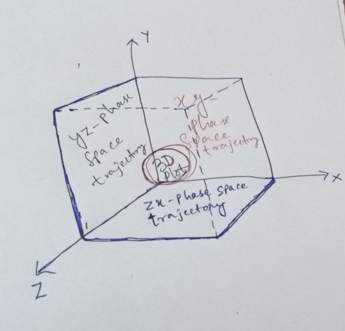
I can plot all these trajectories individually. But I want to plot all these four diagrams in a single figure just like the schematic diagram I have shown below.

Can anybody tell me how to do this?

Answer 1

s = NDSolve[{Derivative[1][x][t] == -0.4*x[t] + y[t] + 10.0*y[t]*z[t],
     Derivative[1][y][t] == -x[t] - 0.4*y[t] + 5.0*x[t]*z[t], 
    Derivative[1][z][t] == 0.175*z[t] - 5.0*x[t]*y[t], x[0] == 0.349, 
    y[0] == 0.0, z[0] == -0.160}, {x, y, z}, {t, 0, 600, 0.01}, 
   MaxSteps -> ∞];

p1 = ParametricPlot3D[Evaluate[{x[t], y[t], z[t]} /. s]
   , {t, 0, 300}
   , PlotRange -> {-1, 1}
   , PlotPoints -> 200
   , AxesLabel -> {Style[x, Medium, Bold, Magenta]
     , Style[y, Medium, Bold, Magenta], 
     Style[z, Medium, Bold(*Plain*), Magenta]}
   , LabelStyle -> Directive[Black, Plain]
   , PlotTheme -> "Scientific"
   , PlotStyle -> Black
   , ImageSize -> 600
   , BoxRatios -> Automatic
   ];

p2 = ParametricPlot3D[Evaluate[{x[t], y[t], -1} /. s]
   , {t, 0, 300}
   , PlotRange -> {-1, 1}
   , PlotPoints -> 1000
   , LabelStyle -> Directive[Black, Plain]
   , PlotStyle -> {Thin, Blue}
   , PlotPoints -> 1000
   , ImageSize -> 600
   , BoxRatios -> Automatic
   ];

p3 = ParametricPlot3D[Evaluate[{-1, y[t], z[t]} /. s]
   , {t, 0, 300}
   , PlotRange -> {-1, 1}
   , PlotPoints -> 1000
   , LabelStyle -> Directive[Black, Plain]
   , PlotStyle -> {Thin, Red}
   , ImageSize -> 600
   , BoxRatios -> Automatic
   ];

p4 = ParametricPlot3D[Evaluate[{x[t], 1, z[t]} /. s]
   , {t, 0, 300}, PlotRange -> {-1, 1}
   , PlotPoints -> 1000
   , LabelStyle -> Directive[Black, Plain]
   , PlotStyle -> {Thin, Darker@Green}
   , ImageSize -> 600
   , BoxRatios -> Automatic
   ];

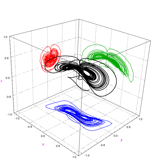
Show[p1, p2, p3, p4
 , ImageSize -> 600
 , Boxed -> True
 , SphericalRegion -> True
 , FaceGrids -> {{0, 1, 0}, {-1, 0, 0}, {0, 0, -1}}
 ]

---

Answer 2

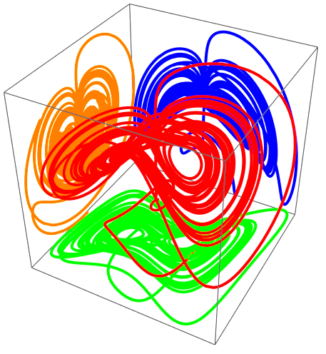
• Using ScalingTransform to project to the three planes.
• Only need p1 in the original code.

{{xmin, xmax}, {ymin, ymax}, {zmin, zmax}} = 
  PlotRange /. AbsoluteOptions[p1, PlotRange];
Graphics3D[{GeometricTransformation[p1[[1]], 
    ScalingTransform[10^-3, {0, 0, 1}, {0, 0, zmin}]] /. 
   Line[pts_] :> {Green, Line[pts]}, 
  GeometricTransformation[p1[[1]], 
    ScalingTransform[10^-3, {0, 1, 0}, {0, ymax, 0}]] /. 
   Line[pts_] :> {Blue, Line[pts]}, 
  GeometricTransformation[p1[[1]], 
    ScalingTransform[10^-3, {1, 0, 0}, {xmin, 0, 0}]] /. 
   Line[pts_] :> {Orange, Line[pts]}, p1[[1]]}]