Plotting Phase Diagram

Question

I have the following problem that I'm sure Mathematica can handle, but it's not working for me!

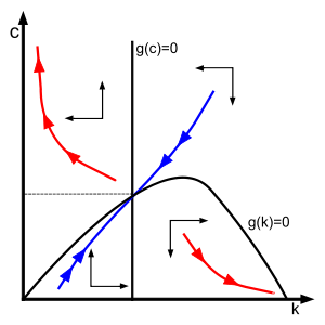
In the following code, I'm trying to replicate the Ramsey Model Phase Diagram.

In fact, I want now to be able to dram the stable arm of the system. My attempted is using NDSolve, since I cannot do better. The idea is given a $z_0$ in the regions where exist a stable arm (the ones where the blue line cuts). I tried the framework of BV problems and add up some 1% range; I'm rather sure Mathematica can do better than this.

Could anybody suggest me a way to solve it, because NDSolve refuses to work with this coding, and I really don't know how to do it.

α = 0.3;
ρ = 0.02;
θ = 2;
η = 0.5;
δ = 0.05;
A = 1.0;

T = 600;
err = 0.01;
{zM, cM} = {250000, 1000};

Dz = A α^α η^η (α+η)^-(α+η) z^(α+η)-δ z- c;
Dc = θ^-1 (A α^α η^η (α+η)^(1-(α+η))  z^(α+η-1) - ρ-δ); 
{zT, cT} = NSolve[{Dc == 0, Dz == 0}, {z, c}][[1, All, 2]]

Plot1 = ContourPlot[{Dz==0,Dc==0},
   {z, 0, zM}, {c, 0, cM},
   PlotTheme -> "Scientific",
   PlotLegends -> {"Subscript[Overscript[z, .], t]=0", "Subscript[Overscript[c, .], t]=0"}, 
   Frame -> False, Axes -> True, AxesLabel -> {"z", "c"},
   PlotRange -> {{0, zM}, {0, cM}}, ImageSize -> Large
 ];

z0 = 10000;

sol=NDSolve[
     {z'[t] == A α^α η^η (α+η)^-(α+η) z[t]^(α+η)- δ z[t]- c[t],
      c'[t] == c[t]/θ (A α^α η^η (α+η)^(1-(α+η)) z[t]^(α+η-1) - ρ-δ),
      Abs[z[T]-zT]<err*zM,
      Abs[c[T]-cT]<err*cM
     },
     {z, c}, {t, 0, T},
     Method -> {"Shooting", "StartingInitialConditions" -> {z[0] == z0}}
    ];

Plot2 = ParametricPlot[Evaluate[{z[t], c[t]} /.sol], {t,0,T},
          PlotRange -> {{0, zM}, {0, cM}}, ImageSize -> Large
        ];

Show[{Plot1, Plot2}]

Answer 1

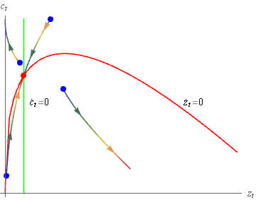
I am badly placed to critic you question since I use to be as criptic as you. First only an economist can understand your objective since this representation is not so standard as you think. I have tried a day long to change the parameters but it is nearly impossible to change the position of c=0. Using the free add-on of Gianluca Gorni here is the best I have been able to do --- I have changed the font to times since I guess you are typesetting with Tex.

Here is the code.

Needs["CurvesGraphics6`"];
ClearAll[α, ρ, θ, η, δ, A, z, c, t];
α = 0.3;
ρ = 0.001;
θ = 2.;
η = 0.09;
δ = 0.05;
 A = 1;
 Φ = 
  A α^α η^η (α + η)^-(α + \
 η);
Ω = 
 A α^α η^η (α + η)^(
 1 - (α + η));
{zM, cM} = {250., 1.}
F[z_, c_] := Φ z^(α + η) - δ z - c
G[z_, c_] := 
1/θ (Ω z^((α + η) - 
  1)) - (ρ + δ)
NSolve[Φ z^(α + η) - δ z == 0, z]
NSolve[1/θ (Ω z^((α + η) - 
   1)) - (ρ + δ) == 0, z]
 sol1 = NDSolve[( {
 {z'[t] == Φ z[t]^(α + η) - δ z[
      t] - c[t]},
 {c'[t] == 
   1/θ (Ω z[t]^((α + η) - 
        1)) - (ρ + δ)},
 {z[0] == 5},
 {c[0] == 1.5}
} ), {z, c}, {t, 0, 800}, PlotSolution -> True, 
ColorFunction -> "DarkRainbow", PlotPoints -> 50];
sol2 = NDSolve[( {
 {z'[t] == Φ z[t]^(α + η) - δ z[
      t] - c[t]},
 {c'[t] == 
   1/θ (Ω z[t]^((α + η) - 
        1)) - (ρ + δ)},
 {z[0] == 15.6342},
 {c[0] == 2}
} ), {z, c}, {t, 0, 100}, PlotSolution -> True, 
ColorFunction -> "DarkRainbow"];
sol3 = NDSolve[( {
 {z'[t] == Φ z[t]^(α + η) - δ z[
      t] - c[t]},
 {c'[t] == 
   1/θ (Ω z[t]^((α + η) - 
        1)) - (ρ + δ)},
 {z[0] == 20},
 {c[0] == 1.2}
 } ), {z, c}, {t, 0, 30}, PlotSolution -> True, 
 ColorFunction -> "DarkRainbow"];
sol4 = NDSolve[( {
 {z'[t] == Φ z[t]^(α + η) - δ z[
      t] - c[t]},
 {c'[t] == 
   1/θ (Ω z[t]^((α + η) - 
        1)) - (ρ + δ)},
 {z[0] == 0.429975},
 {c[0] == .2}
} ), {z, c}, {t, 0, 80}, PlotSolution -> True, 
 ColorFunction -> "DarkRainbow"];
 p = ContourPlot[{F[z, c] == 0, G[z, c] == 0}, {z, 0, 80}, {c, 0, 2.}, 
 AspectRatio -> 0.75, WorkingPrecision -> 20, 
 PlotLegends -> {"\!\(\*SubscriptBox[\(z\), \(t\)]\)=0", 
 "\!\(\*SubscriptBox[\(c\), \(t\)]\)=0"}, Frame -> False, 
  Axes -> True, 
 AxesLabel -> {"\!\(\*SubscriptBox[\(z\), \(t\)]\)", 
 "\!\(\*SubscriptBox[\(c\), \(t\)]\)"}, 
  LabelStyle -> Directive[FontFamily -> "Times"], 
  ContourStyle -> {Red, Green}];
SetOptions[Show, BaseStyle -> {FontFamily -> "Times", FontSize -> 14},
Ticks -> None];
Show[p, sol1[[2]], sol2[[2]], sol3[[2]], sol4[[2]], 
Graphics[{PointSize[0.025], Point[{20, 1.2}, VertexColors -> Blue], 
Point[{15.6342, 2}, VertexColors -> Blue], 
Point[{5, 1.5}, VertexColors -> Blue], 
Point[{0.429975, .2}, VertexColors -> Blue], 
Point[{6.35, 1.355}, VertexColors -> Red]}], 
Graphics[Text[
"\!\(\*SubscriptBox[OverscriptBox[\(c\), \(.\)], \(t\)]\)=0", {12, 
1.05}]], 
Graphics[Text[
"\!\(\*SubscriptBox[OverscriptBox[\(z\), \(.\)], \(t\)]\)=0", {65, 
1.05}]], BaseStyle -> {FontFamily -> "Times", FontSize -> 14}, 
Ticks -> None]

I think that most representations in text books do not emphazises enough on the difficulty of the graphic representations due to numerical problems. One remarks --- I do not know why the graphic her is not exactly the one shown in mathematica --- no labels, no adapted fonts.

A last thing. I have not tried to put the arrows because the graphic could be unreadable.

Nevertheless, if you have difficulties with the code send me a message I will send it to you by mail.