Formatted code
Source Link
MarcoB
  • 67.7k
  • 18
  • 96
  • 197

In fact, I want now to be able to dram the stable arm of the system. My attempted is using NDSOLVENDSolve, since I cannot do better. The idea is given a z0$z_0$ in the regions where exist a stable arm (the ones where the blue line cuts). I tried the framework of BV problems and add up some 1% range; I'm rather sure Mathematica can do better than this.

Could anybody suggest me a way to solve it, because NDSOLVENDSolve refuses to work with this coding, and I really don't know how to do it.

\[Alpha]=0α = 0.3;
\[Rho]=0ρ = 0.02;
\[Theta]=2;θ = 2;
\[Eta]=0η = 0.5;
\[Delta]=0δ = 0.05;
A=1A = 1.0;

T=600;T = 600;
err=0err = 0.01;
{zM, cM} = {250000, 1000};

Dz = A \[Alpha]^\[Alpha]α^α \[Eta]^\[Eta]η^η (\[Alpha]+\[Eta]α+η)^-(\[Alpha]+\[Eta]α+η) z^(\[Alpha]+\[Eta]α+η)-\[Delta]δ z- c;
Dc = \[Theta]^θ^-1 (A \[Alpha]^\[Alpha]α^α \[Eta]^\[Eta]η^η (\[Alpha]+\[Eta]α+η)^(1-(\[Alpha]+\[Eta]α+η))  z^(\[Alpha]+\[Eta]α+η-1) - \[Rho]ρ-\[Delta]δ);  
{zT, cT}=NSolve[ = NSolve[{Dc==0Dc == 0,Dz==0 Dz == 0}, {z, c}][[1, All, 2]]

Plot1 = ContourPlot[{Dz==0,Dc==0},
   {z, 0, zM}, {c, 0, cM},
   PlotTheme ->"Scientific"> "Scientific",
   PlotLegends -> {"Subscript[Overscript[z, .], t]=0", "Subscript[Overscript[c, .], t]=0"}, 
   Frame -> False, Axes ->True> True, AxesLabel -> {"z", "c"},
   PlotRange -> {{0, zM}, {0, cM}}, ImageSize ->Large];> Large
 ];

z0 = 10000;

sol=NDSolve[
     {z'[t]==Az'[t] \[Alpha]^\[Alpha]== \[Eta]^\[Eta]A α^α η^η (\[Alpha]+\[Eta]α+η)^-(\[Alpha]+\[Eta]α+η) z[t]^(\[Alpha]+\[Eta]α+η)- \[Delta]δ z[t]- c[t],
c'[t]==c[t]      c'[t] == c[t]/\[Theta]θ (A \[Alpha]^\[Alpha]α^α \[Eta]^\[Eta]η^η (\[Alpha]+\[Eta]α+η)^(1-(\[Alpha]+\[Eta]α+η)) z[t]^(\[Alpha]+\[Eta]α+η-1) - \[Rho]ρ-\[Delta]δ),
      Abs[z[T]-zT]<err*zM,
      Abs[c[T]-cT]<err*cM
     },
     {z, c}, {t, 0, T},
     Method -> {"Shooting", "StartingInitialConditions" -> {z[0]==z0z[0] == z0}}
    ];

Plot2=ParametricPlot[Evaluate[Plot2 = ParametricPlot[Evaluate[{z[t], c[t]} /.sol],
  {t,0,T},
          PlotRange -> {{0, zM}, {0, cM}}, ImageSize ->Large];> Large
        ];

Show[{Plot1, Plot2}]

Thank you all in advance for you time and expertise.

Best,

In fact, I want now to be able to dram the stable arm of the system. My attempted is using NDSOLVE, since I cannot do better. The idea is given a z0 in the regions where exist a stable arm (the ones where the blue line cuts). I tried the framework of BV problems and add up some 1% range; I'm rather sure Mathematica can do better than this.

Could anybody suggest me a way to solve it, because NDSOLVE refuses to work with this coding, and I really don't know how to do it.

\[Alpha]=0.3;
\[Rho]=0.02;
\[Theta]=2;
\[Eta]=0.5;
\[Delta]=0.05;
A=1.0;

T=600;
err=0.01;
{zM,cM}={250000,1000};

Dz = A \[Alpha]^\[Alpha] \[Eta]^\[Eta] (\[Alpha]+\[Eta])^-(\[Alpha]+\[Eta]) z^(\[Alpha]+\[Eta])-\[Delta] z- c;
Dc = \[Theta]^-1 (A \[Alpha]^\[Alpha] \[Eta]^\[Eta] (\[Alpha]+\[Eta])^(1-(\[Alpha]+\[Eta]))  z^(\[Alpha]+\[Eta]-1) - \[Rho]-\[Delta]); {zT, cT}=NSolve[{Dc==0,Dz==0},{z,c}][[1,All,2]]

Plot1 = ContourPlot[{Dz==0,Dc==0},
{z,0,zM}, {c,0,cM},
PlotTheme ->"Scientific",
PlotLegends ->{"Subscript[Overscript[z, .], t]=0","Subscript[Overscript[c, .], t]=0"}, 
Frame-> False, Axes->True, AxesLabel->{"z","c"},
PlotRange->{{0,zM},{0,cM}}, ImageSize->Large];

z0 = 10000;

sol=NDSolve[
{z'[t]==A \[Alpha]^\[Alpha] \[Eta]^\[Eta] (\[Alpha]+\[Eta])^-(\[Alpha]+\[Eta]) z[t]^(\[Alpha]+\[Eta])- \[Delta] z[t]- c[t],
c'[t]==c[t]/\[Theta] (A \[Alpha]^\[Alpha] \[Eta]^\[Eta] (\[Alpha]+\[Eta])^(1-(\[Alpha]+\[Eta])) z[t]^(\[Alpha]+\[Eta]-1) - \[Rho]-\[Delta]),
Abs[z[T]-zT]<err*zM,
Abs[c[T]-cT]<err*cM},
{z,c}, {t,0,T},
Method->{"Shooting", "StartingInitialConditions"->{z[0]==z0}}];

Plot2=ParametricPlot[Evaluate[{z[t],c[t]} /.sol],
 {t,0,T},
PlotRange->{{0,zM},{0,cM}}, ImageSize->Large];

Show[{Plot1, Plot2}]

Thank you all in advance for you time and expertise.

Best,
In fact, I want now to be able to dram the stable arm of the system. My attempted is using NDSolve, since I cannot do better. The idea is given a $z_0$ in the regions where exist a stable arm (the ones where the blue line cuts). I tried the framework of BV problems and add up some 1% range; I'm rather sure Mathematica can do better than this.

Could anybody suggest me a way to solve it, because NDSolve refuses to work with this coding, and I really don't know how to do it.

α = 0.3;
ρ = 0.02;
θ = 2;
η = 0.5;
δ = 0.05;
A = 1.0;

T = 600;
err = 0.01;
{zM, cM} = {250000, 1000};

Dz = A α^α η^η (α+η)^-(α+η) z^(α+η)-δ z- c;
Dc = θ^-1 (A α^α η^η (α+η)^(1-(α+η))  z^(α+η-1) - ρ-δ);  
{zT, cT} = NSolve[{Dc == 0, Dz == 0}, {z, c}][[1, All, 2]]

Plot1 = ContourPlot[{Dz==0,Dc==0},
   {z, 0, zM}, {c, 0, cM},
   PlotTheme -> "Scientific",
   PlotLegends -> {"Subscript[Overscript[z, .], t]=0", "Subscript[Overscript[c, .], t]=0"}, 
   Frame -> False, Axes -> True, AxesLabel -> {"z", "c"},
   PlotRange -> {{0, zM}, {0, cM}}, ImageSize -> Large
 ];

z0 = 10000;

sol=NDSolve[
     {z'[t] == A α^α η^η (α+η)^-(α+η) z[t]^(α+η)- δ z[t]- c[t],
      c'[t] == c[t]/θ (A α^α η^η (α+η)^(1-(α+η)) z[t]^(α+η-1) - ρ-δ),
      Abs[z[T]-zT]<err*zM,
      Abs[c[T]-cT]<err*cM
     },
     {z, c}, {t, 0, T},
     Method -> {"Shooting", "StartingInitialConditions" -> {z[0] == z0}}
    ];

Plot2 = ParametricPlot[Evaluate[{z[t], c[t]} /.sol], {t,0,T},
          PlotRange -> {{0, zM}, {0, cM}}, ImageSize -> Large
        ];

Show[{Plot1, Plot2}]
Source Link

Plotting Phase Diagram

I have the following problem that I'm sure Mathematica can handle, but it's not working for me!

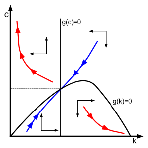
In the following code, I'm trying to replicate the Ramsey Model Phase Diagram.

Ramsey Model Phase Diagram

In fact, I want now to be able to dram the stable arm of the system. My attempted is using NDSOLVE, since I cannot do better. The idea is given a z0 in the regions where exist a stable arm (the ones where the blue line cuts). I tried the framework of BV problems and add up some 1% range; I'm rather sure Mathematica can do better than this.

Could anybody suggest me a way to solve it, because NDSOLVE refuses to work with this coding, and I really don't know how to do it.

\[Alpha]=0.3;
\[Rho]=0.02;
\[Theta]=2;
\[Eta]=0.5;
\[Delta]=0.05;
A=1.0;

T=600;
err=0.01;
{zM,cM}={250000,1000};

Dz = A \[Alpha]^\[Alpha] \[Eta]^\[Eta] (\[Alpha]+\[Eta])^-(\[Alpha]+\[Eta]) z^(\[Alpha]+\[Eta])-\[Delta] z- c;
Dc = \[Theta]^-1 (A \[Alpha]^\[Alpha] \[Eta]^\[Eta] (\[Alpha]+\[Eta])^(1-(\[Alpha]+\[Eta]))  z^(\[Alpha]+\[Eta]-1) - \[Rho]-\[Delta]); {zT, cT}=NSolve[{Dc==0,Dz==0},{z,c}][[1,All,2]]

Plot1 = ContourPlot[{Dz==0,Dc==0},
{z,0,zM}, {c,0,cM},
PlotTheme ->"Scientific",
PlotLegends ->{"Subscript[Overscript[z, .], t]=0","Subscript[Overscript[c, .], t]=0"}, 
Frame-> False, Axes->True, AxesLabel->{"z","c"},
PlotRange->{{0,zM},{0,cM}}, ImageSize->Large];

z0 = 10000;

sol=NDSolve[
{z'[t]==A \[Alpha]^\[Alpha] \[Eta]^\[Eta] (\[Alpha]+\[Eta])^-(\[Alpha]+\[Eta]) z[t]^(\[Alpha]+\[Eta])- \[Delta] z[t]- c[t],
c'[t]==c[t]/\[Theta] (A \[Alpha]^\[Alpha] \[Eta]^\[Eta] (\[Alpha]+\[Eta])^(1-(\[Alpha]+\[Eta])) z[t]^(\[Alpha]+\[Eta]-1) - \[Rho]-\[Delta]),
Abs[z[T]-zT]<err*zM,
Abs[c[T]-cT]<err*cM},
{z,c}, {t,0,T},
Method->{"Shooting", "StartingInitialConditions"->{z[0]==z0}}];

Plot2=ParametricPlot[Evaluate[{z[t],c[t]} /.sol],
{t,0,T},
PlotRange->{{0,zM},{0,cM}}, ImageSize->Large];

Show[{Plot1, Plot2}]

Thank you all in advance for you time and expertise.

Best,