How to plot phase space diagram of a response/slave system of a chaotic attractor?

Question

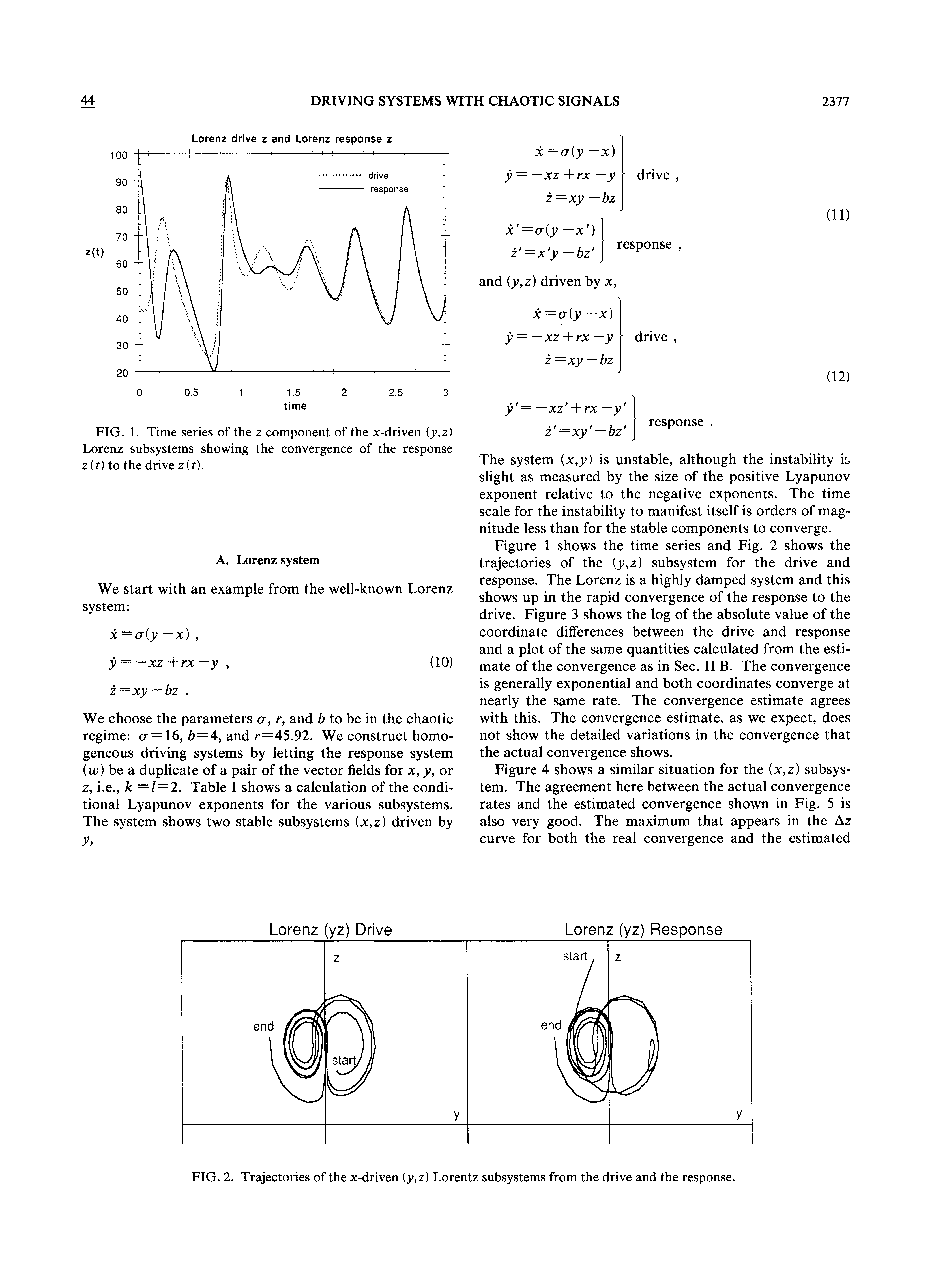
In this attached image, we can see that the Lorenz chaotic attractor can show Master-Slave (Drive-Response)configuration where the Master/Drive system is driven by either y cordinate or x-coorinate.In this attached image, the differential equations for both the cases are given.

Using NDSolve and ParametricPlot3D, I am getting drive system of Lorenz attractor with initial condition $(x0=0,y0=1,z0=0)$ and the code is given below.

solution = 
  NDSolve[{x'[t] == 16 (y[t] - x[t]), 
    y'[t] == 45.92 x[t] - y[t] - x[t] z[t], 
    z'[t] == x[t] y[t] - 4 z[t], x[0] == z[0] == 0, y[0] == 1}, {x, y,
     z}, {t, 0, 32, 0.0001}];
ParametricPlot3D[Evaluate[{x[t], y[t], z[t]} /. solution], {t, 0, 32},
  PlotTheme -> "Scientific", PlotStyle -> Blue, ImageSize -> Small, 
 PlotRange -> Full]

But, I am unable to plot phase space diagram of slave system of this Lorenz system and the differential equations of slave system is given in attached image. As we can see , the slave system consists of 3-variables, but provided equations are 2 only. We know, we can solve equations if and only if no. of equations $>=$ no. of variables.

But, in this attached paper, we can see it is possible to get phase space diagram of slave system also. I do not know how to get this and which information is missing. Using NDSolve , I am not getting any result. What to do to solve slave system?

Answer 1

It looks like the response involves two new variables, e.g., called y' and z' in Eq. 12 of the paper. If that's the correct interpretation, you'll need to solve the "response" part of the equations with a second NDSolve, substituting x[t] from the first and picking initial values for y' and z'.

For example, using y1 and z1 for y' and z' in the response:

responseEqns = With[{b = 4, r = 45.92}, 
  {y1'[t] == -x[t] z1[t] + r x[t] - y1[t], z1'[t] == x[t] y1[t] - b z1[t]}
];

then solve with a choice of initial values for y1 and z1:

response = NDSolve[
   Join[responseEqns /. solution[[1]], {y1[0] == 0, z1[0] == 1}], 
   {y1, z1}, {t, 0, 32, 0.0001}];

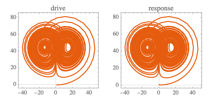
A plot similar to Fig. 2 comparing drive (y,z) and response (y1,z1) is

GraphicsRow[{
  ParametricPlot[Evaluate[{y[t], z[t]} /. solution], {t, 0, 32}, 
   PlotTheme -> "Scientific", ImageSize -> Small, PlotRange -> Full, 
   PlotLabel -> "drive"],
  ParametricPlot[Evaluate[{y1[t], z1[t]} /. response], {t, 0, 32}, 
   PlotTheme -> "Scientific", ImageSize -> Small, PlotRange -> Full, 
   PlotLabel -> "response"]
  }]

which gives

Or you could combine all five equations in a single NDSolve.