6
$\begingroup$

Bug introduced in 13.1 and fixed in 13.2.0


I am trying to compute a deformation and a stress of a material with a custom material law. I have successfully computed the deformation using SolidMechanicsPDEComponent and NDSolveValue. Now I would like to compute and visualize the stress. I have to compute the strain using SolidMechanicsStrain first, which works fine. However the SolidMechanicsStress then sometimes returns, that the stress is zero, which is wrong.

Here is a part of my code:

strain = SolidMechanicsStrain[vars, pars, displacement];

cauchy = SolidMechanicsStress[vars, Join[pars, <|"OutputStressMeasure" -> "Cauchy"|>], strain, displacement];
firstPK = SolidMechanicsStress[vars, Join[pars, <|"OutputStressMeasure" -> "FirstPiolaKirchhoff"|>], strain, displacement];

vars are variables, pars are parameters, displacement is a displacement computed using NDSolveValue.

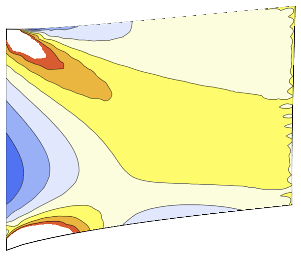
Here is a the visualization of one of the components of the Cauchy stress tensor. All other components are also equal to zero. The first Piola-Kirchhoff is also equal to zero.

ContourPlot[cauchy[[1, 1]], {x, y} ∈ deformedMesh, PlotRange -> All, PlotLegends -> Automatic]

This is the visualization of the computed Cauchy stress tensor. All other components are also equal to zero.

Here are other parts of the code:

ClearAll["Global`*"]
Needs["NDSolve`FEM`"]

coords = {x, y};
deformation = {u[x, y], v[x, y]};

Young = 10^9;
ν = 1/3;

n = 1.5;
α = Pi/4;
Q = {{Cos[α], -Sin[α]}, {Sin[α], Cos[α]}};

GetK[Young_, ν_] := Young/(3*(1 - 2*ν));
GetM[Young_, ν_] := Young*(1 - ν)/((1 + ν)*(1 - 2* ν));
GetG[Young_, ν_] := Young/(2*(1 + ν));

K = GetK[Young, ν];
M = GetM[Young, ν];
G = GetG[Young, ν];

rectangle = Rectangle[{0, 0}, {1, 1}];
mesh = ToElementMesh[rectangle];
vars = {deformation, coords};

pars = <|"MaterialModelFunction" -> QRElasticity, "ModelForm" -> "PlaneStrain", "Thickness" -> 1, "ConstitutiveStressMeasure" -> "FirstPiolaKirchhoff", "MassDensity" -> 980, "BulkModulus" -> K, "PWaveModulus" -> M, "ShearModulus" -> G, "n" -> n, "Q" -> Q|>;
pdeQRElasticity = SolidMechanicsPDEComponent[vars, pars];
pde = {pdeQRElasticity == SolidBoundaryLoadValue[x == 1, vars, pars, <|"Pressure" -> {p, 0}|>], DirichletCondition[{u[x, y] == 0}, x == 0], DirichletCondition[{v[x, y] == 0}, x == 0]};

AbsoluteTiming[displacement = NDSolveValue[pde /. p -> 300000000, {u, v}, {x, y} \[Element] mesh];]
deformedMesh = ElementMeshDeformation[mesh, displacement, "ScalingFactor" -> 1];

The QRElasticity is the custom material law for fiber-reinforced materials. The parameter n describes, how much more stiffer are fibres than the material. The matrix Q is a matrix of rotation that describes the orientation of fibres in the material.

QRElasticity[vars_, pars_, data_] := Module[{u, x, dim, idm, n, Q, K, M, G, F, FAni, R, sinθ, cosθ, a, b, γ, U, RU, δ, ε, pi, σ, τ, STilde11, STilde22, STilde12, STilde, UInvTrans, stressMatrix},

  u = vars[[1]];
  x = vars[[-1]];
  
  K = pars["BulkModulus"];
  M = pars["PWaveModulus"];
  G = pars["ShearModulus"];
  n = pars["n"];
  Q = pars["Q"];
  
  dim = Length[u];
  idm = IdentityMatrix[dim];
  
  (*Print["K = ",K];
  Print["M = ",M];
  Print["G = ",G];*)
  
  F = ConstantArray[0, {dim, dim}];
  F[[1 ;; dim, 1 ;; dim]] = idm + Grad[u, x];
  
  FAni = Q . F . Inverse[Q];
  
  (*Print["F =",F//MatrixForm];
  Print["FAni =",FAni//MatrixForm];*)
  
  R = ConstantArray[0, {dim, dim}];
  sinθ = -FAni[[2, 1]]/Sqrt[FAni[[1, 1]]^2 + FAni[[2, 1]]^2];
  cosθ = FAni[[1, 1]]/Sqrt[FAni[[1, 1]]^2 + FAni[[2, 1]]^2];
  R = {{cosθ, sinθ}, {-sinθ, cosθ}};
  
  (*Print["R = ",R//MatrixForm];*)
  
  a = Sqrt[FAni[[1, 1]]^2 + FAni[[2, 1]]^2];
  b = (FAni[[1, 1]] FAni[[2, 2]] - FAni[[1, 2]] FAni[[2, 1]])/Sqrt[FAni[[1, 1]]^2 + FAni[[2, 1]]^2];
  γ = (FAni[[1, 1]] FAni[[1, 2]] + FAni[[2, 1]] FAni[[2, 2]])/(FAni[[1, 1]]^2 + FAni[[2, 1]]^2);
  U = {{a, a*γ}, {0, b}};
  
  (*Print["U = ",U//MatrixForm];*)
  
  (*Print["RU = ",Simplify[R.U]//MatrixForm];*)
  
  δ = Log[Sqrt[a^n*b^(1/n)]];
  ε = Log[Sqrt[(a^n)/(b^(1/n))]];
  
  (*Print["delta = ",δ];
  Print["epsilon = ",ε];*)
  
  pi = 4*K*δ;
  σ = 2*M*ε;
  τ = G*γ;
  
  STilde11 = 1/2*(n*pi + n*σ);
  STilde22 = 1/2*(pi/n - σ/n);
  STilde12 = (b/a)*τ;
  STilde = {{STilde11, STilde12}, {STilde12, STilde22}};
  
  (*Print["STilde = ",STilde//MatrixForm];*)
  
  UInvTrans = Inverse[Transpose[U]];
  
  (*Print["UInvTrans = ", UInvTrans//MatrixForm];*)
  
  stressMatrix = Inverse[Q] . R . STilde . UInvTrans . Q;
  
  stressMatrix = Simplify[stressMatrix[[1 ;; dim, 1 ;; dim]]];
  
  (*Print["StressMatrix = ", stressMatrix//MatrixForm];*)
  
  stressMatrix
  
  ]
$\endgroup$
5
  • $\begingroup$ You did not define: vars, pars, displacement, deformedMesh $\endgroup$ Commented Sep 20, 2022 at 13:25
  • $\begingroup$ I did, I just didnt post it here. I will edit the post to contain more code. $\endgroup$
    – lemurman
    Commented Sep 20, 2022 at 13:29
  • 1
    $\begingroup$ Can you share your QRElasticity? People will need the full code to experiment with this. $\endgroup$
    – user21
    Commented Sep 20, 2022 at 15:52
  • 1
    $\begingroup$ No problem. I have eddited the post. $\endgroup$
    – lemurman
    Commented Sep 20, 2022 at 16:49
  • 1
    $\begingroup$ This is a bug. I am currently trying to figure out if there is a workaround. $\endgroup$
    – user21
    Commented Sep 22, 2022 at 13:17

2 Answers 2

3
$\begingroup$

The behavior you see is caused by a bug. A simplified version of the bug is the following:

m1 = {{1, 2}, {3, 4}};
m2 = {{0, 0}, {0, 0}};
sa1 = SymmetrizedArray[m1];
sa2 = SymmetrizedArray[m2];

Normal[sa1 + sa2]
(* {{0, 0}, {0, 0}} *)

The expected result is:

m1 + m2
(* {{1, 2}, {3, 4}} *)

Now, you can see that for:

m1 = {{1, 2}, {3, 4}};
m2 = {{$MachineEpsilon, 0}, {0, $MachineEpsilon}};
sa1 = SymmetrizedArray[m1];
sa2 = SymmetrizedArray[m2];
Normal[(sa1 + sa2)]
(* {{1., 2}, {3, 4.}} *)

we get more or less what we are looking for. This will be the basis for the workaround. The problem comes up because an initial stress is added to the computed stress. The default initial stress is 0, but if we specify a stress of size $MachineEpsilon we can extract the stress from the SolidMechanicsStress function.

Before we do that, however, I'd like to point out a few other things you may not be aware of. First, to get the embedding dimension you use

dim = Length[u];

it would be a bit better to use

dim = Length[x];

You may have more dependent variables than just the ones your interested (maybe an additional pressure). The spatial dimension of x is saver way to get to the dimension.

Another thing that is useful is to look at the default parameters:

PDEModels`DefaultModelParameters[vars, pars, "SolidMechanics"]

This will give an association of parameters which will contain the default values and some additionally defined values.

pars = <|"MaterialModelFunction" -> QRElasticity, 
   "ModelForm" -> "PlaneStrain", "Thickness" -> 1, 
   "ConstitutiveStressMeasure" -> "FirstPiolaKirchhoff", 
   "MassDensity" -> 980, "BulkModulus" -> K, "PWaveModulus" -> M, 
   "ShearModulus" -> G, "n" -> n, "Q" -> Q
   |>;

PDEModels`DefaultModelParameters[vars, pars, "SolidMechanics"]

In your original case this gives:

Out[22]= <|"MaterialModelFunction" -> QRElasticity, 
 "ModelForm" -> "PlaneStrain", "Thickness" -> 1, 
 "ConstitutiveStressMeasure" -> "FirstPiolaKirchhoff", 
 "MassDensity" -> 980, "BulkModulus" -> 1000000000, 
 "PWaveModulus" -> 1500000000, "ShearModulus" -> 375000000, 
 "n" -> 1.5, 
 "Q" -> {{1/Sqrt[2], -(1/Sqrt[2])}, {1/Sqrt[2], 1/Sqrt[2]}}, 
 "VectorLength" -> 3, "EmbeddingDimension" -> 2, 
 "MaterialModel" -> "Custom", "GeometricNonlinearity" -> True, 
 "EngineeringStrain" -> False, "StrainMeasure" -> "Infinitesimal", 
 "EquilibriumStressMeasure" -> "Cauchy", 
 "StrainFunction" -> SolidMechanicsStrain, 
 "StressFunction" -> SolidMechanicsStress|>

The default for a "Custom" material model is to use an "Infinitesimal" strain measure. I am wondering if you meant to use a "GreenLargange" strain measure? Depending on what you are going to say to this I might revise my decision about the default.

OK, let's look at a setup of pars, that I think does what you want:

pars = <|"MaterialModelFunction" -> QRElasticity, 
   "ModelForm" -> "PlaneStrain", "Thickness" -> 1, 
   "ConstitutiveStressMeasure" -> "FirstPiolaKirchhoff", 
   "MassDensity" -> 980, "BulkModulus" -> K, "PWaveModulus" -> M, 
   "ShearModulus" -> G, "n" -> n, "Q" -> Q,
   "InitialStress" -> {$MachineEpsilon, $MachineEpsilon},
   "StrainMeasure" -> "GreenLagrange"
   |>;

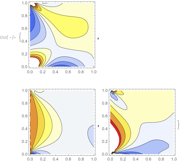
I have added a minute InitialStress to work around the bug and a GreenLagrange strain measure. With that I get a different strain (well I have asked for that) and a stress that is non-zero.

ContourPlot[#, {x, y} \[Element] mesh, 
   ColorFunction -> "TemperatureMap"] & /@ {strain[[1, 1]], 
  strain[[2, 2]], strain[[1, 2]]}

enter image description here

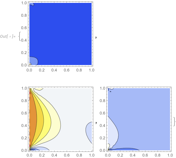
You can add the option PlotRange->All to eliminate the cut off of extreme values:

ContourPlot[#, {x, y} \[Element] mesh, 
   ColorFunction -> "TemperatureMap", PlotRange -> All] & /@ {strain[[
   1, 1]], strain[[2, 2]], strain[[1, 2]]}

enter image description here

Then for the stress:

stress = 
 SolidMechanicsStress[vars, 
  Join[pars, <|"OutputStressMeasure" -> "Cauchy"|>], strain,
  displacement]

The fact that you have to specify the OutputStressMeasure for a custom material model is something that could work automatically. It should just use a Cauchy stress as a default. Any opinion on that?

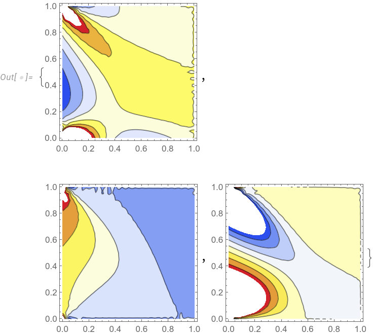
The stress now has the minute $MachineEpsilon on the diagional but that's not important and visualization works:

ContourPlot[#, {x, y} \[Element] mesh, 
   ColorFunction -> "TemperatureMap"] & /@ {stress[[1, 1]], 
  stress[[2, 2]], stress[[1, 2]]}

enter image description here

Update:

Again, you can use PlotRange->All

enter image description here

The PK1 you can use:

SolidMechanicsStress[vars, 
 Join[pars, <|
   "OutputStressMeasure" -> "FirstPiolaKirchhoff"|>], strain,
 displacement]

For PK2 you currently need to do this (which is fixed in the upcoming version 13.2)

 (* S = F^-1.P *)
 PDEModels`StructuralMechanicsDump`StressMeasureConversion[
  "FirstPiolaKirchhoff", "SecondPiolaKirchhoff", 
  pk1Stress_, {U : {__}, ___, X : {__}}, pars_] :=
 Module[{f, pk2Stress}, f = Grad[U, X] + IdentityMatrix[Length[X]]; 
  pk2Stress = Inverse[f] . pk1Stress; pk2Stress]

SolidMechanicsStress[vars, 
 Join[pars, <|
   "OutputStressMeasure" -> "SecondPiolaKirchhoff"|>], strain,
 displacement]

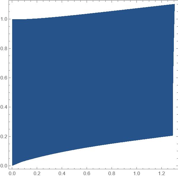
To visualize the Cauchy $\sigma_{11}$ stress in the deformed mesh use:

cauchy = 
  SolidMechanicsStress[vars, 
   Join[pars, <|"OutputStressMeasure" -> "Cauchy"|>], strain,
   displacement];
deformedCauchy11 = 
  ElementMeshInterpolation[deformedMesh, 
   Chop[cauchy[[1, 1]]][[0]]["ValuesOnGrid"]];
Show[
 ToBoundaryMesh[deformedMesh]["Wireframe"],
 ContourPlot[deformedCauchy11[x, y], {x, y} \[Element] deformedMesh, 
  ColorFunction -> "TemperatureMap"]
 ]

enter image description here

I apologize for the inconvenience and thank you for reporting this.

$\endgroup$
12
  • $\begingroup$ Thank you for your answer. It looks like this workaround works. But there is still one problem. The Cauchy stress tensor is in actual configuration, not referential, so I would like to visualize it in the deformed mesh. However the ContourPlot for some reason cuts the plot at x = 1 and y = 1, so the plot isn't completely visible. $\endgroup$
    – lemurman
    Commented Sep 22, 2022 at 20:46
  • $\begingroup$ And to answer your questions about stress and strain measures: 1. I am not intrested in the strain (at least for now), so I don't care about the default choice. But you are probably right that Green-Lagrange makes more sense in my case. 2. I am aware that the Cauchy is the default choice, but I am also interested in other stresses so I added the "OutputStressMeasure" -> "Cauchy" to make the code more constistent. $\endgroup$
    – lemurman
    Commented Sep 22, 2022 at 20:46
  • $\begingroup$ And another problem I have is that an attempt to compute the second Piola-Kirchhoff stress tensor via "OutputStressMeasure "->" SecondPiolaKirchhoff" results in error. $\endgroup$
    – lemurman
    Commented Sep 22, 2022 at 21:05
  • $\begingroup$ You mean like this $\endgroup$
    – user21
    Commented Sep 22, 2022 at 21:07
  • 1
    $\begingroup$ Thank you for your help and offer. I will definitely send you an email soon. $\endgroup$
    – lemurman
    Commented Sep 23, 2022 at 11:47
3
$\begingroup$

We made in this code only small modification like $K\rightarrow K0$, since K is a symbol occupied by system.

ClearAll["Global`*"]
Needs["NDSolve`FEM`"]

coords = {x, y};
deformation = {u[x, y], v[x, y]};

Young = 10^9;
\[Nu] = 1/3;

n = 1.5;
\[Alpha] = Pi/4;
Q = {{Cos[\[Alpha]], -Sin[\[Alpha]]}, {Sin[\[Alpha]], Cos[\[Alpha]]}};

GetK[Young_, \[Nu]_] := Young/(3*(1 - 2*\[Nu]));
GetM[Young_, \[Nu]_] := 
  Young*(1 - \[Nu])/((1 + \[Nu])*(1 - 2*\[Nu]));
GetG[Young_, \[Nu]_] := Young/(2*(1 + \[Nu]));

K0 = GetK[Young, \[Nu]];
M = GetM[Young, \[Nu]];
G = GetG[Young, \[Nu]];
QRElasticity[vars_, pars_, data_] := 
 Module[{u, x, dim, idm, n, Q, K0, M, G, F, FAni, R, sin\[Theta], 
   cos\[Theta], a, b, \[Gamma], U, RU, \[Delta], \[CurlyEpsilon], 
   pi, \[Sigma], \[Tau], STilde11, STilde22, STilde12, STilde, 
   UInvTrans, stressMatrix}, u = vars[[1]];
  x = vars[[-1]];
  K0 = pars["BulkModulus"];
  M = pars["PWaveModulus"];
  G = pars["ShearModulus"];
  n = pars["n"];
  Q = pars["Q"];
  dim = Length[u];
  idm = IdentityMatrix[dim];
  (*Print["K = ",K];
  Print["M = ",M];
  Print["G = ",G];*)F = ConstantArray[0, {dim, dim}];
  F[[1 ;; dim, 1 ;; dim]] = idm + Grad[u, x];
  FAni = Q . F . Inverse[Q];
  (*Print["F =",F//MatrixForm];
  Print["FAni =",FAni//MatrixForm];*)
  R = ConstantArray[0, {dim, dim}];
  sin\[Theta] = -FAni[[2, 1]]/Sqrt[FAni[[1, 1]]^2 + FAni[[2, 1]]^2];
  cos\[Theta] = FAni[[1, 1]]/Sqrt[FAni[[1, 1]]^2 + FAni[[2, 1]]^2];
  R = {{cos\[Theta], sin\[Theta]}, {-sin\[Theta], cos\[Theta]}};
  (*Print["R = ",R//MatrixForm];*)
  a = Sqrt[FAni[[1, 1]]^2 + FAni[[2, 1]]^2];
  b = (FAni[[1, 1]] FAni[[2, 2]] - FAni[[1, 2]] FAni[[2, 1]])/
    Sqrt[FAni[[1, 1]]^2 + FAni[[2, 1]]^2];
  \[Gamma] = (FAni[[1, 1]] FAni[[1, 2]] + 
      FAni[[2, 1]] FAni[[2, 2]])/(FAni[[1, 1]]^2 + FAni[[2, 1]]^2);
  U = {{a, a*\[Gamma]}, {0, b}};
  (*Print["U = ",U//MatrixForm];*)(*Print["RU = ",Simplify[R.U]//
  MatrixForm];*)\[Delta] = Log[Sqrt[a^n*b^(1/n)]];
  \[CurlyEpsilon] = Log[Sqrt[(a^n)/(b^(1/n))]];
  (*Print["delta = ",\[Delta]];
  Print["epsilon = ",\[CurlyEpsilon]];*)pi = 4*K0*\[Delta];
  \[Sigma] = 2*M*\[CurlyEpsilon];
  \[Tau] = G*\[Gamma];
  STilde11 = 1/2*(n*pi + n*\[Sigma]);
  STilde22 = 1/2*(pi/n - \[Sigma]/n);
  STilde12 = (b/a)*\[Tau];
  STilde = {{STilde11, STilde12}, {STilde12, STilde22}};
  stressMatrix = Inverse[Q] . R . STilde . UInvTrans . Q;
  stressMatrix = Simplify[stressMatrix[[1 ;; dim, 1 ;; dim]]];
  stressMatrix]
rectangle = Rectangle[{0, 0}, {1, 1}];
mesh = ToElementMesh[rectangle];
vars = {deformation, coords};
strain = SolidMechanicsStrain[vars, pars, displacement];

cauchy = 
  SolidMechanicsStress[vars, 
   Join[pars, <|"OutputStressMeasure" -> "Cauchy"|>], strain, 
   displacement];
firstPK = 
  SolidMechanicsStress[vars, 
   Join[pars, <|"OutputStressMeasure" -> "FirstPiolaKirchhoff"|>], 
   strain, displacement];
pars = <|"MaterialModelFunction" -> QRElasticity, 
   "ModelForm" -> "PlaneStrain", "Thickness" -> 1, 
   "ConstitutiveStressMeasure" -> "FirstPiolaKirchhoff", 
   "MassDensity" -> 980, "BulkModulus" -> K0, "PWaveModulus" -> M, 
   "ShearModulus" -> G, "n" -> n, "Q" -> Q|>;
pdeQRElasticity = SolidMechanicsPDEComponent[vars, pars];
pde = {pdeQRElasticity == 
    SolidBoundaryLoadValue[x == 1, vars, 
     pars, <|"Pressure" -> {p, 0}|>], 
   DirichletCondition[{u[x, y] == 0}, x == 0], 
   DirichletCondition[{v[x, y] == 0}, x == 0]};

AbsoluteTiming[
 displacement = 
   NDSolveValue[
    pde /. p -> 300000000, {u, v}, {x, y} \[Element] mesh];]
deformedMesh = 
 ElementMeshDeformation[mesh, displacement, "ScalingFactor" -> 1];

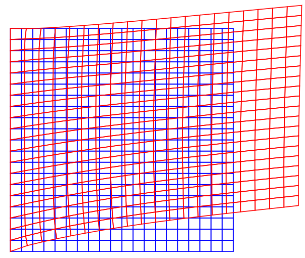
Visualization. Deformed mesh

Show[mesh["Wireframe"["MeshElementStyle" -> EdgeForm[Blue]]], 
 deformedMesh["Wireframe"["MeshElementStyle" -> EdgeForm[Red]]]]

Figure 1

Strain

{ContourPlot[strain[[1, 1]], {x, y} \[Element] rectangle, 
  PlotRange -> All, PlotLegends -> Automatic, 
  ColorFunction -> "Rainbow", Contours -> 20, ContourStyle -> White, 
  PlotLabel -> 
   "\!\(\*FormBox[\(\*SubscriptBox[\(\[Epsilon]\), \(x\
\[InvisibleSpace]x\)]\(\\\ \)\),
TraditionalForm]\)"], 
 ContourPlot[strain[[1, 2]], {x, y} \[Element] rectangle, 
  PlotRange -> All, PlotLegends -> Automatic, 
  ColorFunction -> "Rainbow", Contours -> 20, ContourStyle -> White, 
  PlotLabel -> 
   "\!\(\*FormBox[\(\*SubscriptBox[\(\[Epsilon]\), \(x\
\[InvisibleSpace]y\)]\(\\\ \)\),
TraditionalForm]\)"], 
 ContourPlot[strain[[2, 2]], {x, y} \[Element] rectangle, 
  PlotRange -> All, PlotLegends -> Automatic, 
  ColorFunction -> "Rainbow", Contours -> 20, ContourStyle -> White, 
  PlotLabel -> 
   "\!\(\*FormBox[\(\*SubscriptBox[\(\[Epsilon]\), \(y\
\[InvisibleSpace]y\)]\(\\\ \)\),
TraditionalForm]\)"]}

Figure 2

We also can use stressMatrix to visualize the first Piola-Kirchhoff tensor as follows

ClearAll["Global`*"]
Needs["NDSolve`FEM`"]
QRElasticity[vars_, pars_, data_] := 
 Module[{u, x, dim, idm, n, Q, K0, M, G, F, FAni, R, sin\[Theta], 
   cos\[Theta], a, b, \[Gamma], U, RU, \[Delta], \[CurlyEpsilon], 
   pi, \[Sigma], \[Tau], STilde11, STilde22, STilde12, STilde, 
   UInvTrans, stressMatrix}, u = vars[[1]];
  x = vars[[-1]];
  K0 = pars["BulkModulus"];
  M = pars["PWaveModulus"];
  G = pars["ShearModulus"];
  n = pars["n"];
  Q = pars["Q"];
  dim = Length[u];
  idm = IdentityMatrix[dim];
  (*Print["K = ",K];
  Print["M = ",M];
  Print["G = ",G];*)F = ConstantArray[0, {dim, dim}];
  F[[1 ;; dim, 1 ;; dim]] = idm + Grad[u, x];
  FAni = Q . F . Inverse[Q];
  (*Print["F =",F//MatrixForm];
  Print["FAni =",FAni//MatrixForm];*)
  R = ConstantArray[0, {dim, dim}];
  sin\[Theta] = -FAni[[2, 1]]/Sqrt[FAni[[1, 1]]^2 + FAni[[2, 1]]^2];
  cos\[Theta] = FAni[[1, 1]]/Sqrt[FAni[[1, 1]]^2 + FAni[[2, 1]]^2];
  R = {{cos\[Theta], sin\[Theta]}, {-sin\[Theta], cos\[Theta]}};
  (*Print["R = ",R//MatrixForm];*)
  a = Sqrt[FAni[[1, 1]]^2 + FAni[[2, 1]]^2];
  b = (FAni[[1, 1]] FAni[[2, 2]] - FAni[[1, 2]] FAni[[2, 1]])/
    Sqrt[FAni[[1, 1]]^2 + FAni[[2, 1]]^2];
  \[Gamma] = (FAni[[1, 1]] FAni[[1, 2]] + 
      FAni[[2, 1]] FAni[[2, 2]])/(FAni[[1, 1]]^2 + FAni[[2, 1]]^2);
  U = {{a, a*\[Gamma]}, {0, b}};
  (*Print["U = ",U//MatrixForm];*)(*Print["RU = ",Simplify[R.U]//
  MatrixForm];*)\[Delta] = Log[Sqrt[a^n*b^(1/n)]];
  \[CurlyEpsilon] = Log[Sqrt[(a^n)/(b^(1/n))]];
  (*Print["delta = ",\[Delta]];
  Print["epsilon = ",\[CurlyEpsilon]];*)pi = 4*K0*\[Delta];
  \[Sigma] = 2*M*\[CurlyEpsilon];
  \[Tau] = G*\[Gamma];
  STilde11 = 1/2*(n*pi + n*\[Sigma]);
  STilde22 = 1/2*(pi/n - \[Sigma]/n);
  STilde12 = (b/a)*\[Tau];
  STilde = {{STilde11, STilde12}, {STilde12, STilde22}};
  (*Print["STilde = ",STilde//MatrixForm];*)
  UInvTrans = Inverse[Transpose[U]];
  (*Print["UInvTrans = ",UInvTrans//MatrixForm];*)
  stressMatrix = Inverse[Q] . R . STilde . UInvTrans . Q;
  stressMatrix = Simplify[stressMatrix[[1 ;; dim, 1 ;; dim]]];
  (*Print["StressMatrix = ",stressMatrix//MatrixForm];*)stressMatrix]

coords = {x, y};
deformation = {u[x, y], v[x, y]};
Young = 10^9;
\[Nu] = 1/3;

n = 1.5;
\[Alpha] = Pi/4;
Q = {{Cos[\[Alpha]], -Sin[\[Alpha]]}, {Sin[\[Alpha]], Cos[\[Alpha]]}};

GetK[Young_, \[Nu]_] := Young/(3*(1 - 2*\[Nu]));
GetM[Young_, \[Nu]_] := 
  Young*(1 - \[Nu])/((1 + \[Nu])*(1 - 2*\[Nu]));
GetG[Young_, \[Nu]_] := Young/(2*(1 + \[Nu]));

K0 = GetK[Young, \[Nu]];
M = GetM[Young, \[Nu]];
G = GetG[Young, \[Nu]];

rectangle = Rectangle[{0, 0}, {1, 1}];
mesh = ToElementMesh[rectangle];
vars = {deformation, coords};

pars = <|"MaterialModelFunction" -> QRElasticity, 
   "ModelForm" -> "PlaneStrain", "Thickness" -> .01, 
   "ConstitutiveStressMeasure" -> "FirstPiolaKirchhoff", 
   "MassDensity" -> 980, "BulkModulus" -> K0, "PWaveModulus" -> M, 
   "ShearModulus" -> G, "n" -> n, "Q" -> Q|>;
pdeQRElasticity = SolidMechanicsPDEComponent[vars, pars];
strain = SolidMechanicsStrain[vars, pars, deformation]; cauchy = 
 SolidMechanicsStress[vars, 
  Join[pars, <|"OutputStressMeasure" -> "Cauchy"|>], strain, 
  deformation]; firstPK = 
 SolidMechanicsStress[vars, 
  Join[pars, <|"OutputStressMeasure" -> "FirstPiolaKirchhoff"|>], 
  strain, deformation];
pde = {pdeQRElasticity == 
    SolidBoundaryLoadValue[x == 1, vars, 
     pars, <|"Pressure" -> {p, 0}|>], 
   DirichletCondition[{u[x, y] == 0}, x == 0], 
   DirichletCondition[{v[x, y] == 0}, x == 0]};

sol = NDSolve[pde /. p -> 300000000, {u, v}, {x, y} \[Element] mesh];

Visualization

pars0 = <|"MassDensity" -> 980, "BulkModulus" -> K0, 
   "PWaveModulus" -> M, "ShearModulus" -> G, "n" -> n, "Q" -> Q|>;

PK1=QRElasticity[vars, pars0, 0] /. sol[[1]];

{ContourPlot[PK1[[1, 1]], {x, y} \[Element] rectangle, 
  PlotRange -> All, PlotLegends -> Automatic, 
  ColorFunction -> "Rainbow", Contours -> 20, ContourStyle -> White, 
  PlotLabel -> "FirstPiolaKirchhoff11"], 
 ContourPlot[PK1[[1, 2]], {x, y} \[Element] rectangle, 
  PlotRange -> All, PlotLegends -> Automatic, 
  ColorFunction -> "Rainbow", Contours -> 20, ContourStyle -> White, 
  PlotLabel -> "FirstPiolaKirchhoff12"], 
 ContourPlot[PK1[[2, 2]], {x, y} \[Element] rectangle, 
  PlotRange -> All, PlotLegends -> Automatic, 
  ColorFunction -> "Rainbow", Contours -> 20, ContourStyle -> White, 
  PlotLabel -> "FirstPiolaKirchhoff22"]}

Figure 3

$\endgroup$
10
  • $\begingroup$ Thank you for your answer. However I think your solution also doesn't work. 1. Visualization of any other component of Cauchy stress tensor than [1,2] results in blank picture. 2. The first Piola-Kirchhoff stress tensor remains the same even if the deformation is different. For example changing the parameter 'n' from 1.5 to 1 results in different deformation, but the picture remains the same. $\endgroup$
    – lemurman
    Commented Sep 21, 2022 at 14:28
  • $\begingroup$ Actually, this is your code. Do you ask me to improve your code so that we can compute all stress components? Then, please, can you provide model in Latex as well? $\endgroup$ Commented Sep 21, 2022 at 15:07
  • $\begingroup$ I would like to be able to compute the stress (ideally the norm of the stress tensors, but if I am able to compute the components, then I am able to compute the norm), which now does not work. Right now this particular model is not written anywhere, because it is a modification (generalization) of another model. However I am sure that the model (in the code represented by the QRElasticity module) is correct. $\endgroup$
    – lemurman
    Commented Sep 21, 2022 at 16:16
  • $\begingroup$ This line is under question stressMatrix = Inverse[Q] . R . STilde . UInvTrans . Q. $\endgroup$ Commented Sep 21, 2022 at 16:27
  • $\begingroup$ The stressMatrix is the first Piola-Kirchhoff tensor, which is equal to the Kirchhoff tensor S times the transposed inverse of deformation gradient F. This model uses the QR decomposition of the deformation gradient (matrices R and U). The relation for the Kirchhoff stress tensor comes from the article "Stress / strain basis pairs for anisotropic materials" by Erel and Freed. The matrix Q is a matrix that describes the direction of fibres in material. $\endgroup$
    – lemurman
    Commented Sep 21, 2022 at 19:21

Your Answer

By clicking “Post Your Answer”, you agree to our terms of service and acknowledge you have read our privacy policy.

Not the answer you're looking for? Browse other questions tagged or ask your own question.