Large deformation of solids

Question

Link to notebook with this question and code

I'd like to understand how large deformations of solid mechanics work and how they are implemented. For this am looking at the following reference problem: A long slender beam is fixated at the left. A larger force is pushing in the negative x direction and a smaller force in the negative y direction.

To keep things a simple as possible this example uses a linear plane stress model (a linear material model) - it's just about the large deformation.

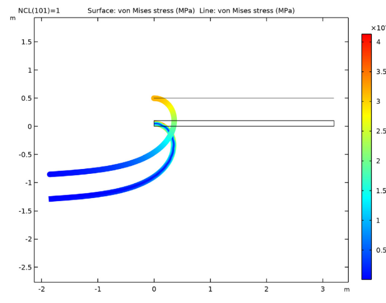
A reference to this benchmark problem can be found here. There is also a video starting at time 28:00. Geometric nonlinearity is explained at 26:22.

The result for the plane stress case is a largely deformed beam. In the picture below (taken from the source given above) we are talking about the lower of the two beams.

Set up some parameters.

Needs["NDSolve`FEM`"]
length = 3.2;
hight = 1/10;
thickness = 1/10;
Ω = Rectangle[{0, 0}, {length, hight}];
mesh = ToElementMesh[Ω];
bmesh = ToBoundaryMesh[mesh];

The total force is given. I am not 100% sure what total force means in Comsol speak, but I assume it means force per area. The force in the negative x direction is 10^3 times larger then the one in the negative y direction. We use Poisson's ratio of 0 and Young's modulus of 210 GPa.

(*force per area*)
fx = -3.844*10^6/(hight*thickness);
fy = fx*10^-3;
bc2 = {NeumannValue[fx, x == length], NeumannValue[fy, x == length]};
bc1 = DirichletCondition[{u[x, y] == 0, v[x, y] == 0}, x == 0];
materialData = {nu -> 0, Y -> 210*10^9};

We start by using a linear - no large deformation - plane stress operator used on SE in several places and known to produce correct results. The only thing I changed is adding a 'thickness' factor to account for the thickness that is not 1.

PlaneStress[{Y_, nu_}, {u_, v_}, X : {x_, y_}] := Module[{pStress},
  (* uses global thickness *)
  pStress = -thickness * 
    Y/(1 - nu^2)*{{{{1, 0}, {0, (1 - nu)/2}}, {{0, nu}, {(1 - nu)/2, 
        0}}}, {{{0, (1 - nu)/2}, {nu, 0}}, {{(1 - nu)/2, 0}, {0, 1}}}};
  {Inactive[Div][pStress[[1, 1]] . Inactive[Grad][u, X], X] + 
    Inactive[Div][pStress[[1, 2]] . Inactive[Grad][v, X], X], 
   Inactive[Div][pStress[[2, 1]] . Inactive[Grad][u, X], X] + 
    Inactive[Div][pStress[[2, 2]] . Inactive[Grad][v, X], X]}]

Solve the equation:

planeStress = 
  PlaneStress[{Y, nu} /. materialData, {u[x, y], v[x, y]}, {x, y}];
{uif2, vif2} = 
  NDSolveValue[{planeStress == bc2, bc1}, {u, 
    v}, {x, y} ∈ Ω];
Show[bmesh["Wireframe"],
 deform2 = 
  ElementMeshDeformation[mesh, {uif2, vif2}, "ScalingFactor" -> 1][
   "Wireframe"["MeshElementStyle" -> EdgeForm[Red]]]]

Next, I am solving the same problem with a different setup. This setup will allow me later to easily change to a large deformation setup. We use the following:

This is then converted to a 2 by 2 matrix:

Normal[
 SymmetrizedArray[
  Thread[Rule[{{1, 1}, {2, 2}, {1, 2}}, {Subscript[σ, xx], 
     Subscript[σ, yy], Subscript[τ, xy]}]], Automatic, 
  Symmetric]]

(* {{Subscript[σ, xx], Subscript[τ, 
  xy]}, {Subscript[τ, xy], Subscript[σ, yy]}} *)

And plugged into (with an additional thickness factor):

Table[
 Inactive[Div][-{{Subscript[σ, xx], Subscript[τ, 
      xy]}, {Subscript[τ, xy], Subscript[σ, 
      yy]}}[[i, ;;]], X], {i, Length[U]}]

(* {Inactive[
   Div][{-Subscript[σ, xx], -Subscript[τ, xy]}, {x, y}], 
 Inactive[Div][{-Subscript[τ, xy], -Subscript[σ, yy]}, {x,
    y}]} *)


makeStressModel[e_] := Block[
  {materialData, materialModel, exx, eyy, gxy, eVec, strain, nu, Y, 
   stress},
  (* linear elastic plane stress model *)
  
  materialModel = 
   Y/(1 - nu^2)*{{1, nu, 0}, {nu, 1, 0}, {0, 0, (1 - nu)/2}};
  exx = e[[1, 1]];
  eyy = e[[2, 2]];
  gxy = (e[[1, 2]] + e[[2, 1]]);
  (* for plane stress ezz =nu/(1-nu)*(exx+
  eyy) does not play a role since nu = 0 *)
  strain = {exx, eyy, gxy};
  stress = (materialModel . strain);
  Normal[SymmetrizedArray[
    Thread[Rule[{{1, 1}, {2, 2}, {1, 2}}, stress]], Automatic, 
    Symmetric]]
  ]


(* uses global defined thickness *)
makePDEModel[stressMatrix_] := 
 Table[Inactive[Div][-thickness*stressMatrix[[i, ;;]], X], {i, 
   Length[U]}]

We verify that this gives the same results as a the previous plane stress operator:

X = {x, y};
U = {u[x, y], v[x, y]};

(* geometric linear *)
gu = Grad[U, X];
gut = Transpose[gu];
e = 1/2 (gu + gut);
stress = makeStressModel[e];

pde = makePDEModel[stress /. materialData];
{uif, vif} = 
  NDSolveValue[{pde == bc2, bc1}, {u, v}, {x, y} ∈ mesh];

Show[bmesh["Wireframe"],
 deform1 = 
  ElementMeshDeformation[mesh, {uif, vif}, "ScalingFactor" -> 1][
   "Wireframe"["MeshElementStyle" -> EdgeForm[Brown]]]]

Norm[uif["ValuesOnGrid"] - uif2["ValuesOnGrid"]]
Norm[vif["ValuesOnGrid"] - vif2["ValuesOnGrid"]]

(* 1.43378*10^-10
6.49507*10^-9*)

With the framework in place and verified, I want to look at the large deformations. I set up the deformation gradient f and set up the non-linear strain.

(* geometric nonlinear *)
f = Grad[U, {x, y}] + IdentityMatrix[2];
e1 = 1/2 (Transpose[f] . f - IdentityMatrix[2]) // Expand // Simplify;

With the same approach as above

stress = makeStressModel[e1];
pde = makePDEModel[stress /. materialData];
{uif, vif} = 
  NDSolveValue[{pde == bc2, bc1}, {u, 
    v}, {x, y} ∈ Ω];
mesh = uif["ElementMesh"];
Show[ToBoundaryMesh[mesh]["Wireframe"],
 deform2 = 
  ElementMeshDeformation[mesh, {uif, vif}, "ScalingFactor" -> 1][
   "Wireframe"["MeshElementStyle" -> EdgeForm[Red]]]]

Show[deform1, deform2]

This is not correct. I would have expected a failure from the nonlinear solver for the large deformation or a much larger deformation. I am trying to understand what I am missing. Question: Why is this approach wrong or where did I make a mistake?

A second way to specify the large strains is by

gu = Grad[U, X];
gut = Transpose[gu];
e2 = 1/2 (gu + gut + gut . gu);
FullSimplify[e1 - e2]

(* {{0, 0}, {0, 0}} *)

But it gives the same result. I have verified that the PDE coefficients parse correctly

{state} = 
  NDSolve`ProcessEquations[{pde == bc2, bc1}, {u, 
    v}, {x, y} ∈ Ω];
GetInactivePDE[state] - pde

(*{0, 0}*)

The next idea was that using the Cauchy stress is not correct. So I changed to the second Piola-Kirchhoff stress. We compute the stress as before

stress = makeStressModel[e1];

Now, find the deformation gradient, it's inverse and transpose and J the determinant of f.

f = Grad[U, X] + IdentityMatrix[2];
invF = Inverse[f];
invFT = Transpose[invF];
piolaStress = Det[f]*invF . stress . invFT;
pde = makePDEModel[piolaStress /. materialData];
{uif, vif} = 
  NDSolveValue[{pde == bc2, bc1}, {u, 
    v}, {x, y} ∈ Ω];
deform3 = 
  ElementMeshDeformation[mesh, {uif, vif}, "ScalingFactor" -> 1][
   "Wireframe"["MeshElementStyle" -> EdgeForm[Blue]]];
Show[deform2, deform3]

Still, no joy.

{state} = 
  NDSolve`ProcessEquations[{pde == bc2, bc1}, {u, 
    v}, {x, y} ∈ Ω];
GetInactivePDE[state] - pde
(* {0, 0} *)

Link to notebook with this question and code

Update:

From the video I understand that the following is use:

$\nabla \cdot (F S)^T$

The deformation gradient:

$F = \nabla u + I$

The material law (Hooks law): $S = ? F^{-T} (C:\epsilon) F^{-1}$

Here, the $?$ is something I can not read - could be $J = det(F)$

$\epsilon = \frac{1}{2} ((\nabla u)^T + (\nabla u) + (\nabla u)^T*(\nabla u))$

Answer 1

I think you guys are using the wrong theory, as far as I understood the code above. Sadly I only have little time, and in this answer I can only give you the theory without code. If I read your code wrong and you are using the equivalent correct theory, then I apologize of course :D.

In continuum mechanics of solid bodies, you generally have material points $X$ and spatial positions $x$. The motion is usually defined as $x = \chi(X)$. The gradient of the motion $\chi$ w.r.t. (with respect to) matter is referred to as the deformation gradient $F_{ij}(X) = \partial \chi_i(X) / \partial X_j$.

Small deformations

When you assume small deformations, you implicitly assume $F \approx I$, which imply $x \approx X$. Because of this, you approximate the displacement field of a material point $u(X)$ by $u(x)$ (note the new dependency on spatial position $x$ instead of material point $X$). This yields that the equilibrium condition in terms of the Cauchy stress $\sigma(x)$ $$ \sum_{j=1}^3 \frac{\partial \sigma_{ij}(x)}{\partial x_j} = 0 \ , \quad i=1,\dots,3 $$ w.r.t. space can be solve for linear elasticity with the elastic law $\sigma(x) = \mathbb{C}(x) \varepsilon(x)$, some fourth-order tensor stiffness of space $\mathbb{C}(x)$ (e.g., with isotropic material behavior determined by Young's modulus and Poisson's ratio) and the infinitesimal strain tensor $$ \varepsilon_{ij}(x) = \frac{1}{2}\left( \frac{\partial u_i(x)}{\partial x_j} + \frac{\partial u_j(x)}{\partial x_i} \right). $$ So, for small deformations you have everything parametrized w.r.t. space and you can go as you already now.

Large deformations

For large deformations the situation changes since the general equilibrium equation in terms of the Cauchy stress $\sigma$ $$ \sum_{j=1}^3 \frac{\partial \sigma_{ij}(x)}{\partial x_j} = 0 \ , \quad i=1,\dots,3 $$ is of course still valid, but now you have to take into account the difference between spatial positions $x$ and material points $X$. An easier way to do this is to solve the equivalent equilibrium condition in the reference placement formulated in terms of the first Piola-Kirchohoff stress tensor $P(X)$ [1PK] (note the dependency on matter $X$ and differentiation w.r.t. $X$ and not $x$) $$ \sum_{j=1}^3 \frac{\partial P_{ij}(X)}{\partial X_j} = 0 \ , \quad i=1,\dots,3 $$ see, e.g., equation (4.123) here. The 1PK is connected to the second Piola-Kirchoff stress tensor $S(X)$ [2PK] by $$ P(X) = F(X)S(X) $$ In elasticity of large deformations, usually 2PK is modeled. The analogous elastic law is St.Venant's law $$ S(X) = \mathbb{C}(X)E(X) $$ with Green's strain tensor \begin{equation} E(X) = \frac{1}{2}(F^T(X)F(X) - I) \end{equation} (Side note: St. Venant's law is not always a good idea, it yields unphysical behavior for very large deformations). Now, in order to have a PDE, we need to insert the displacement field $u(X)$ accordingly (note the dependency on matter). Use the relation $$ \chi(X) = X + u(X) $$ in $F(X) = I + \partial u(X)/\partial X$, which then you can put into $E(X)$. This yields the in-$u$-highly-nonlinear PDE $$ \sum_{j=1}^3 \frac{\partial [(I + \partial u(X)/\partial X)(\mathbb{C}(X)\{(I + \partial u(X)/\partial X)^T(I + \partial u(X)/\partial X) - I\}/2)]_{ij}}{\partial X_j} \ , \quad i=1,\dots,3 $$ This is the 3D nonlinear PDE that you should solve in the reference (initial) configuration with BC's described in terms of $X$.

In your PDE, are you sure that the thickness thing really takes care of the rest of the nonlinearity? Seems odd to me, but I am only familiar with the general 3D theory, not with the beam theory for large deformations.

Again, if I read your code wrong and you are using the equivalent correct theory, then I apologize of course.

In terms of physical plausibility of the model the following points are important:

• which strain tensor do they use? Green's strain is fine only for moderate strains. There are alternatives, e.g., Hencky strain.
• which constitutive law (elastic law) is used? St. Venant's law is not applicable for very large strains. There are alternatives, e.g., based on hyperelastic models (stress $P$ or $S$ derived from scalar potential).

Answer 2

It is not 2D problem, but 3D problem. So we actually need some 3D model to describe deformation. But before do this, we can describe the problem in the beam theory. Fortunately, this problem has exact solution - see, for instance, Landau and Lifshitz Theory of Elasticity. Parameters of the problem in the beam theory

inert = .1^4/12; L = 3.2; Y = 2.10 10^11; Fx = 3.84 10^6; 

Maximum angle of deflection

l[t0_?NumericQ] := 
 Sqrt[.5 inert Y/Fx] NIntegrate[1/Sqrt[Cos[t] - Cos[t0]], {t, 0, t0}];
 x0 = x /. FindRoot[l[x] - L == 0, {x, 3.05}]

(*Out[]= 3.0716*) 

Coordinates of beam axis

y[t_] := -Sqrt[2 inert Y/Fx] (Sqrt[1 - Cos[x0]] - 
     Sqrt[Cos[t] - Cos[x0]]);
x[t_?NumericQ] := 
  Sqrt[.5 inert Y/Fx] NIntegrate[
    Cos[tet]/Sqrt[Cos[tet] - Cos[x0]], {tet, 0, t}];

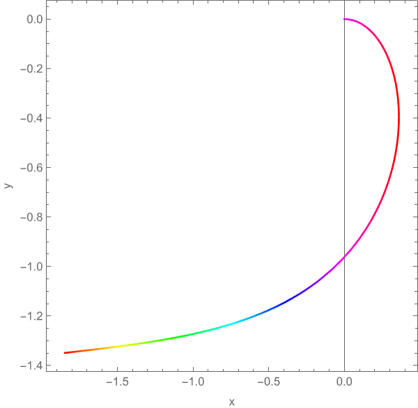
pic1=ParametricPlot[{x[t], y[t]}, {t, 0, x0}, PlotRange -> All, 
 FrameLabel -> {"x", "y"}, AspectRatio -> 1, Frame -> True, 
 ColorFunction -> Hue] 

Final horizontal and vertical displacement at the tip

final = {x[x0]-L, y[x0]}

 {-5.04634, -1.34933}

To compare with COMSOL we look at Table 1, and there are these values refer as follows {-5.05,-1.35}. Now we prepare two functions

v0 = Interpolation[Table[{l[t], y[t]}, {t, .01, x0, .001}]];

u0 = Interpolation[Table[{l[t], x[t] - l[t]}, {t, .01, x0, .001}]];

Let consider linear theory with Dirichletian conditions only

Needs["NDSolve`FEM`"]

x1 = 3.2;
y1 = 1/10;
z1 = 1/10;
reg = Cuboid[{0, 0, 0}, {x1, y1, z1}]; mesh = 
 ToElementMesh[reg, MaxCellMeasure -> 0.00001]
mesh["Wireframe"["MeshElementStyle" -> EdgeForm[Blue]]]

ClearAll[stressOperator];
stressOperator[
  Y_, ν_] := {Inactive[
     Div][{{0, 0, -((Y*ν)/((1 - 2*ν)*(1 + ν)))}, {0, 0, 
       0}, {-Y/(2*(1 + ν)), 0, 0}} . 
     Inactive[Grad][w[x, y, z], {x, y, z}], {x, y, z}] + 
   Inactive[
     Div][{{0, -((Y*ν)/((1 - 2*ν)*(1 + ν))), 
       0}, {-Y/(2*(1 + ν)), 0, 0}, {0, 0, 0}} . 
     Inactive[Grad][v[x, y, z], {x, y, z}], {x, y, z}] + 
   Inactive[
     Div][{{-((Y*(1 - ν))/((1 - 2*ν)*(1 + ν))), 0, 
       0}, {0, -Y/(2*(1 + ν)), 0}, {0, 0, -Y/(2*(1 + ν))}} . 
     Inactive[Grad][u[x, y, z], {x, y, z}], {x, y, z}], 
  Inactive[Div][{{0, 0, 0}, {0, 
       0, -((Y*ν)/((1 - 
              2*ν)*(1 + ν)))}, {0, -Y/(2*(1 + ν)), 0}} . 
     Inactive[Grad][w[x, y, z], {x, y, z}], {x, y, z}] + 
   Inactive[
     Div][{{0, -Y/(2*(1 + ν)), 
       0}, {-((Y*ν)/((1 - 2*ν)*(1 + ν))), 0, 0}, {0, 0, 
       0}} . Inactive[Grad][u[x, y, z], {x, y, z}], {x, y, z}] + 
   Inactive[
     Div][{{-Y/(2*(1 + ν)), 0, 
       0}, {0, -((Y*(1 - ν))/((1 - 2*ν)*(1 + ν))), 0}, {0,
        0, -Y/(2*(1 + ν))}} . 
     Inactive[Grad][v[x, y, z], {x, y, z}], {x, y, z}], 
  Inactive[Div][{{0, 0, 0}, {0, 
       0, -Y/(2*(1 + ν))}, {0, -((Y*ν)/((1 - 
              2*ν)*(1 + ν))), 0}} . 
     Inactive[Grad][v[x, y, z], {x, y, z}], {x, y, z}] + 
   Inactive[
     Div][{{0, 0, -Y/(2*(1 + ν))}, {0, 0, 
       0}, {-((Y*ν)/((1 - 2*ν)*(1 + ν))), 0, 0}} . 
     Inactive[Grad][u[x, y, z], {x, y, z}], {x, y, z}] + 
   Inactive[
     Div][{{-Y/(2*(1 + ν)), 0, 0}, {0, -Y/(2*(1 + ν)), 0}, {0,
        0, -((Y*(1 - ν))/((1 - 2*ν)*(1 + ν)))}} . 
     Inactive[Grad][w[x, y, z], {x, y, z}], {x, y, z}]}
peram = {Y -> 210 10^1, ν -> 0.0};(*We don't use load, therefore scale of Y taken as arbitrary*)

Solution and visualization

{U, V, W} = 
  NDSolveValue[{stressOperator[Y, ν] == {0, 0, 0}, 
     DirichletCondition[{u[x, y, z] == 0, v[x, y, z] == 0, 
       w[x, y, z] == 0}, x == 0], 
     DirichletCondition[{u[x, y, z] == u0[x], v[x, y, z] == v0[x]}, 
      1.06 <= x <= x0], 
     DirichletCondition[{u[x, y, z] == -5.05, v[x, y, z] == -1.35}, 
      x == x1]} /. peram, {u, v, w}, {x, y, z} ∈ mesh];

Show[{mesh["Wireframe"["MeshElementStyle" -> EdgeForm[Gray]]], 
  ElementMeshDeformation[mesh, {U, V, W}][
   "Wireframe"[
    "ElementMeshDirective" -> 
     Directive[EdgeForm[Blue], FaceForm[]]]]}, Axes -> True, 
 AxesLabel -> {x, y, z}]

It looks nice, but there is a message

ElementMesh::femimq: The element mesh has insufficient quality of -0.967913. A quality estimate below 0. may be caused by a wrong ordering of element incidents or self-intersecting elements.

Now we can turn to the nonlinear case. First we verifier 2D linear model

Needs["NDSolve`FEM`"]
length = 3.2;
hight = 1/10;
thickness = 1/10;
\[CapitalOmega] = Rectangle[{0, 0}, {length, hight}];
mesh = ToElementMesh[\[CapitalOmega]]
bmesh = ToBoundaryMesh[mesh];
(*force per area*)
fx = -3.844*10^6/(hight*thickness);
fy = fx*10^-3;
bc2 = {NeumannValue[fx, x == length], NeumannValue[fy, x == length]};
bc1 = {DirichletCondition[{u[x, y] == 0, v[x, y] == 0}, x == 0], 
   DirichletCondition[{u[x, y] == u0[x], v[x, y] == v0[x]}, 
    1.06 <= x <= x0], 
   DirichletCondition[{u[x, y] == -5.05, v[x, y] == -1.35}, 
    x == length]};
materialData = {nu -> 0., Y -> 210*10^9};

makeStressModel[e_] := Block[
  {materialData, materialModel, exx, eyy, gxy, eVec, strain, nu, Y, 
   stress},
  (* linear elastic plane stress model *)
  materialModel = 
   Y/(1 - nu^2)*{{1, nu, 0}, {nu, 1, 0}, {0, 0, (1 - nu)/2}};
  exx = e[[1, 1]];
  eyy = e[[2, 2]];
  gxy = (e[[1, 2]] + e[[2, 1]]);
  (* for plane stress ezz =nu/(1-nu)*(exx+
  eyy) does not play a role since nu = 0 *)
  strain = {exx, eyy, gxy};
  stress = (materialModel . strain);
  Normal[SymmetrizedArray[
    Thread[Rule[{{1, 1}, {2, 2}, {1, 2}}, stress]], Automatic, 
    Symmetric]]
  ]

(* uses global defined thickness *)
makePDEModel[stressMatrix_] := 
 Table[Inactive[Div][-thickness*stressMatrix[[i, ;;]], X], {i, 
   Length[U]}]

X = {x, y};
U = {u[x, y], v[x, y]};
(* geometric linear *)
gu = Grad[U, X];
gut = Transpose[gu];
e = 1/2 (gu + gut);
stress = makeStressModel[e];
pde = makePDEModel[stress /. materialData];
{uif, vif} = 
  NDSolveValue[{pde == {0, 0}, bc1}, {u, v}, {x, y} \[Element] mesh];
pic2=Show[bmesh["Wireframe"],
 deform1 = 
  ElementMeshDeformation[mesh, {uif, vif}, "ScalingFactor" -> 1][
   "Wireframe"["MeshElementStyle" -> EdgeForm[Brown]]]]

As result we have nice picture and same message as above

ElementMesh::femimq: The element mesh has insufficient quality of -0.966859. A quality estimate below 0. may be caused by a wrong ordering of element incidents or self-intersecting elements.

Nevertheless we can compare the beam theory and linear theory combining Figure 1 and Figure 3 in one plot as Show[pic2, pic1]

It looks like a perfect agreement. No wonder since we use the beam theory solution as input in a form of bc1. Finally we try to solve nonlinear model. Note, that in this case we use the first and last points of the beam theory in bc1

Needs["NDSolve`FEM`"]
length = 3.2;
hight = 1/10;
thickness = 1/10;
\[CapitalOmega] = Rectangle[{0, 0}, {length, hight}];
mesh = ToElementMesh[\[CapitalOmega]]
bmesh = ToBoundaryMesh[mesh];

(*force per area*)
fx = -3.844*10^6/(hight*thickness);
fy = fx*10^-3;
bc2 = {NeumannValue[fx, x == length], NeumannValue[fy, x == length]};
bc1 = {DirichletCondition[{u[x, y] == 0, v[x, y] == 0}, x == 0], 
   DirichletCondition[{u[x, y] == -5.05, v[x, y] == -1.35}, 
    x == length]};
materialData = {nu -> 0., Y -> 210*10^9};

makeStressModel[e_] := Block[
  {materialData, materialModel, exx, eyy, gxy, eVec, strain, nu, Y, 
   stress},
  (* linear elastic plane stress model *)
  materialModel = 
   Y/(1 - nu^2)*{{1, nu, 0}, {nu, 1, 0}, {0, 0, (1 - nu)/2}};
  exx = e[[1, 1]];
  eyy = e[[2, 2]];
  gxy = (e[[1, 2]] + e[[2, 1]]);
  (* for plane stress ezz =nu/(1-nu)*(exx+
  eyy) does not play a role since nu = 0 *)
  strain = {exx, eyy, gxy};
  stress = (materialModel . strain);
  Normal[SymmetrizedArray[
    Thread[Rule[{{1, 1}, {2, 2}, {1, 2}}, stress]], Automatic, 
    Symmetric]]
  ] 
X = {x, y};
U = {u[x, y], v[x, y]};

(* uses global defined thickness *)
makePDEModel[stressMatrix_] := 
 Table[Inactive[Div][-thickness*stressMatrix[[i, ;;]], X], {i, 
   Length[U]}]

(* geometric nonlinear *)
f = Grad[U, {x, y}] + IdentityMatrix[2];
e1 = 1/2 (Transpose[f] . f - IdentityMatrix[2]) // Expand // Simplify;

stress = makeStressModel[e1];
pde = makePDEModel[stress /. materialData];
{uif, vif} = 
  NDSolveValue[{pde == {0, 0}, bc1}, {u, v}, {x, y} \[Element] mesh];
pic3 = Show[ToBoundaryMesh[mesh]["Wireframe"],
  deform2 = 
   ElementMeshDeformation[mesh, {uif, vif}, "ScalingFactor" -> 1][
    "Wireframe"["MeshElementStyle" -> EdgeForm[Red]]]]

The picture below looks different from the linear and beam theory as well

Show[pic3, pic1]

Also we have a message

ElementMesh::femimq: The element mesh has insufficient quality of -0.00267866. A quality estimate below 0. may be caused by a wrong ordering of element incidents or self-intersecting elements.

Finally we can test the second Piola-Kirchhoff stress model on the moving grid as follows

Needs["NDSolve`FEM`"]
length = 3.2;
hight = 1/10;
thickness = 1/10;
\[CapitalOmega] = Rectangle[{0, 0}, {length, hight}];
mesh[0] = ToElementMesh[\[CapitalOmega]];
bmesh[0] = ToBoundaryMesh[mesh[0]]; 
LL[0] = Line[Take[bmesh[0][[1]], -5]];

(*force per area*)
fx = -3.844*10^6/(hight*thickness);
fy = fx*10^-3;
bc1[0] = {DirichletCondition[{u[x, y] == 0, v[x, y] == 0}, x == 0]};
materialData = {nu -> 0., Y -> 210*10^9};

makeStressModel[e_] := Block[
  {materialData, materialModel, exx, eyy, gxy, eVec, strain, nu, Y, 
   stress},
  (* linear elastic plane stress model *)
  materialModel = 
   Y/(1 - nu^2)*{{1, nu, 0}, {nu, 1, 0}, {0, 0, (1 - nu)/2}};
  exx = e[[1, 1]];
  eyy = e[[2, 2]];
  gxy = (e[[1, 2]] + e[[2, 1]]);
  (* for plane stress ezz =nu/(1-nu)*(exx+
  eyy) does not play a role since nu = 0 *)
  strain = {exx, eyy, gxy};
  stress = (materialModel . strain);
  Normal[SymmetrizedArray[
    Thread[Rule[{{1, 1}, {2, 2}, {1, 2}}, stress]], Automatic, 
    Symmetric]]
  ]

X = {x, y};
U = {u[x, y], v[x, y]};

(* uses global defined thickness *)
makePDEModel[stressMatrix_] := 
 Table[Inactive[Div][-thickness*stressMatrix[[i, ;;]], X], {i, 
   Length[U]}]

(* geometric nonlinear *)
f = Grad[U, {x, y}] + IdentityMatrix[2];
e1 = 1/2 (Transpose[f] . f - IdentityMatrix[2]) // Expand // Simplify;
stress = makeStressModel[e1];
pde = makePDEModel[stress /. materialData]; invF = Inverse[f];
invFT = Transpose[invF];
piolaStress = 1/Det[f]*invF . stress . invFT;
pde1 = makePDEModel[piolaStress /. materialData];

n = 100; bc2[0] = {NeumannValue[fx , Element[{x, y}, LL[0]]], 
  NeumannValue[fy , Element[{x, y}, LL[0]]]}; Do[{uif[i], vif[i]} = 
  NDSolveValue[{pde1 == bc2[i - 1]/n, bc1[0]}, {u, 
    v}, {x, y} \[Element] mesh[i - 1]];
 mesh[i] = ElementMeshDeformation[mesh[i - 1], {uif[i], vif[i]}]; 
 bmesh[i] = ToBoundaryMesh[mesh[i]]; 
 LL[i] = Line[Take[bmesh[i][[1]], -5]]; 
 bc2[i] = {NeumannValue[fx , Element[{x, y}, LL[i]]], 
   NeumannValue[fy , Element[{x, y}, LL[i]]]};, {i, 20}]

Table[Show[ToBoundaryMesh[mesh[0]]["Wireframe"], 
  mesh[i]["Wireframe"["MeshElementStyle" -> EdgeForm[Red]]], 
  pic1], {i, 20}] 

Note, this model is not correlated well with the beam theory. But it gives large deformation in iteration process with our arbitrary choice. Therefore if we add time then this model probably can be useful.