(NLM @ Circular TimeSeries model ) == invalid phase confidence intervals

Question

In the realm of TimeSeries of data with Circular Statistics, NonlinearModelFit (NLM) correctly generates reasonable Standard Error & confidence intervals for phase parameters (phaseCIs) with x-values that are integer offsets from a reference time (TRef). However, when AbsoluteTime values are utilized, resulting NLM Standard Error for phaseCIs are nonsensical. NOTE: I'm aware of FittedModel::constr warning, but still...

Questions:

1. Why does NLM ignore parameter constraints Abs[phi] <= 2Pi when AbsoluteTime units are utilized?
2. Is there an additional NLM tuning parameter to ensure Phi never steps outside its constrained param value?
3. Is there a two-pass strategy to get reasonable phaseCIs (e.g., estimate BestFitParameters in one pass with a specific NLM Method, and then run a second NLM passing with a Method that explicitly applies parameter constraints)?
4. (More generally) What other issues does NLM have with respect to TimeSeries data with Circular Statistical models?

(* Globals *)
{dayAsSeconds, lunarDayAsSeconds} = 
  QuantityMagnitude @  
     UnitConvert[Quantity[#, "Hours"], "Seconds"] & /@ {24, 24.8};
TRef = DateObject@ {2021, 1, 12, 0, 0} ;
deltaT = 
  QuantityMagnitude @  UnitConvert[Quantity[30, "Minutes"], "Seconds"];
(* Define xValues, one with TRef offset, the other AbsoluteTime *)
xAsOffsets =  Range[5 dayAsSeconds, 20 dayAsSeconds , deltaT ];
xAsAbsoluteTime = 
  AbsoluteTime[TRef + Quantity[#, "Seconds"] ] & /@ xAsOffsets;

NOTE: At this point, the only difference between xAsOffsets and xAsAbsoluteTime is their IntegerLength[] size: the former are offset values from a TRef {0, 3600, ...} with IntegerLength[] <= 7 whereas the latter are AbsoluteTime values {3819830400, 3819832200, ...} whose IntegerLength[] == 10. Both are monotonically increasing by 1800.

(* Model *)
model = M + A1 Cos[2 Pi (t / tau1) + phi1] +   
   A2 Cos[2 Pi (t / tau2) + phi2] ;
modelSeeds =  { M -> 100, A1 -> 10, tau1 -> dayAsSeconds, 
   phi1 -> - Pi/4, A2 -> 2, tau2 -> lunarDayAsSeconds, 
   phi2 -> - Pi/4};
SeedRandom[1];
rnd[dummy_] := 5 RandomReal [{-.5, .5}];
(* Generate xyPairs *)
xyAsOffset = 
  Table[{t, (model /. modelSeeds) + rnd[t]} , {t, xAsOffsets }];
xyAsAbsoluteTime = 
  Table[{t, (model /. modelSeeds) + rnd[t]} , {t, xAsAbsoluteTime }];
(* Prepare NLM wrapper *)
nlmParms = { {M}, {A1}, {tau1, dayAsSeconds}, {phi1, Pi}, {A2}, {tau2,
     lunarDayAsSeconds}, {phi2, Pi}};
nlmConstraint = 
  Abs[phi1] <= 2 Pi && Abs[phi2] <= 2 Pi && A1 > 0 && A2 > 0;
nlm[data_, opts : OptionsPattern[NonlinearModelFit]] := 
 nlm[data, opts] = 
  NonlinearModelFit[data, {model, nlmConstraint}, nlmParms, t, opts];

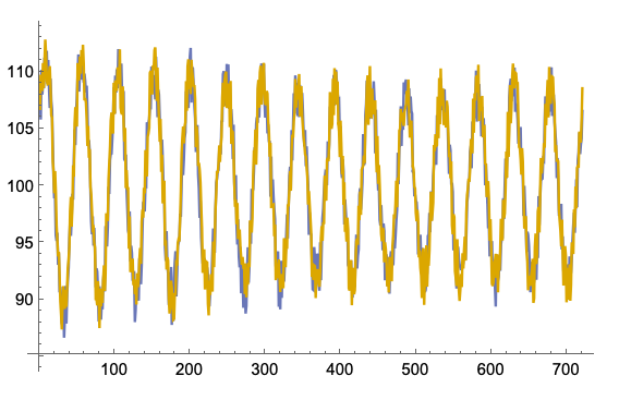
Visually verify both computed dataset Y-values are in the same phase

ListPlot[{xyAsOffset[[All, 2]], xyAsAbsoluteTime[[All, 2]]}, 
 Joined -> True]

Visually compare phi1 and phi2 Standard Error and Confidence Intervals to see the crazy phaseCIs for xyAsAbsoluteTime.

compareCIResults[opts : OptionsPattern[NonlinearModelFit]] := 
 TableForm[{#["ParameterConfidenceIntervalTable"] & /@ {nlm[
      xyAsOffset, opts], nlm[xyAsAbsoluteTime, opts]}}, 
  TableHeadings -> {{opts}, {"xAsOffsetsFromTRef", 
     "xAsAbsoluteTime"}}];
compareCIResults[]

Answer 1

This (for me) has been challenging but in essence, given the data and model, the parameters phi1 and tau1 are almost perfectly correlated (as are phi2 and tau2) which means one can set phi1 and phi2 to any value and you'll get an almost identical fit. So the "crazy" standard errors are due to the overparameterization of the model rather than any error in NonlinearModelFit.

Consider an example that exactly matches your data generation and model.

(* Specify model and parameter values of interest *)
model = m + a1 Cos[2 Pi t/(10^4 tau1) + phi1 ] + 
   a2 Cos[2 Pi t/(10^4 tau2) + phi2 ];
parameters = {m -> 100, a1 -> 10, tau1 -> 8.64, a2 -> 2, 
   tau2 -> 8.928, phi1 -> -π/4, phi2 -> -π/4};

Note that I've scaled tau1 and tau2 so that all parameters are nearly the same order of magnitude which is generally good practice and tends to give one more numerically stable results.

(* Specify predictor values *)
n = 701;
x = 381830400 + 1800 Range[0, n];

(* Generate response *)
SeedRandom[12345];
error = RandomVariate[UniformDistribution[{-2.5, 2.5}], n + 1];
y = (model /. parameters /. t -> x) + error;
xy = Transpose[{x, y}];

(* Fit regression *)
restrictions = {a1 > 0, a2 > 0, tau1 > 0, tau2 > 0};
(* Model fitting all parameters *)
nlm1 = NonlinearModelFit[xy, {model, restrictions}, 
  {{m, 100}, {a1, 10}, {tau1, 8.64}, {phi1, -Pi/4},
     {a2, 2}, {tau2, 8.928}, {phi2, -Pi/4}}, t] // Quiet;
(* Model fixing phi1 and phi2 - doesn't matter what values are used *)   
nlm2 = NonlinearModelFit[xy, {model /. {phi1 -> 1, phi2 -> 1}, restrictions},
    {{m, 100}, {a1, 10}, {tau1, 8.64}, {a2, 2}, {tau2, 8.928}}, t] // Quiet;

The fits are nearly identical.

(* Show results *)
Show[Plot[{nlm1[t], nlm2[t]}, {t, Min[x], Max[x]}, 
  PlotStyle -> {{LightGray, Thickness[0.01]}, {Red, Thickness[0.0005]}}],
  ListPlot[xy], AspectRatio -> 1/4, ImageSize -> Full]

(One fit is in light gray with a wider line and the other fit is in red.)

To justify the claim that phi1 and tau1 (and phi2 and tau2) are nearly perfectly correlated consider the correlation matrix from nlm1 above (where all parameters were fit):

NumberForm[nlm1["CorrelationMatrix"] // MatrixForm, 3]

There are other highly correlated estimators. In fact, all parameters except m are highly correlated with each other which can indicate numerical instability in the estimates of those parameters.