Confidence interval of transformed Fitted Model

Question

I have a FitteddModel coming from a NonlinearModelFit this model depends on two parameters x1 and x2. I want to obtain the values of x2 at which the output of the model is 0.5, for a long list of x1.I do this in the following way:

Table[FindRoot[model[x, y] == 0.5, {y, 1}], {x, -50, 20}]

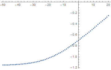
So I can obtain a graph like this:

The problem now is trying to add the errors on every point or a confidence band in the graph. I'm completely clueless about how to do it.

Hope you can help.

Here is the model I'm trying to fit:

K1[ca_] := (10^LogKd)/( (10^(ca))^n)
Kv[v_] := E^(2.8 (v + 18)/25.7)
Po[v_, ca_] := (K1[ca]*Kv[v])/(1 + K1[ca] + (K1[ca]*Kv[v]))
inh[v_, ca_] := Po[v, ca]/Po[v, -5]    
model = NonlinearModelFit[data, inh[x1, x2], {LogKd, n}, {x1, x2}]

The data can be found here

Answer 1

This answer gives how to obtain approximate confidence intervals for y in Solve[inh[x,y]==0.5,y] given x and accounting for the uncertainties in the estimates of LogKd and n from the nonlinear regression using the Delta Method. See https://en.wikipedia.org/wiki/Delta_method and/or

Bishop, Y.M. M., Fienberg, S.E. and Holland, P.W. (1975). 
    Discrete Multivariate Analysis: Theory and Practice. M.I.T. Press, Cambridge, MA.

First perform the regression and obtain estimates of the coefficients and the covariance matrix:

nlm = NonlinearModelFit[data, inh[x1, x2], {LogKd, n}, {x1, x2}]
sol = nlm["BestFitParameters"]
cov = nlm["CovarianceMatrix"]

Now solve for y in terms of x:

f[x_] := y /. Solve[inh[x, y] == 0.5, y][[1]]

Take the partial derivative with respect to both regression parameters:

fpartial = D[f[x], {{LogKd, n}}]

The approximate variance of y given x is given by

yVar = fpartial.cov.fpartial /. sol

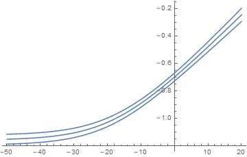
Now plot the prediction and the associated approximate 95% confidence bands:

Plot[{f[x], f[x] + 1.96 yVar^0.5, f[x] - 1.96 yVar^0.5} /. sol, {x, -50, 20}]