2
$\begingroup$

I have a set of data $y_i (z_i)$ with errors $\Delta y_i$, that can be found here

Here

Thus first, I call the data

dataSN = Import["Cat3_0mod.txt", "Table"];
sigdata = dataSN[[All, 4]];
lendata = Length[zdata];

fitSN = Table[{dataSN[[i, 2]], dataSN[[i, 3]]}, {i, 1, lendata}];

I want to fit these data to a complicated model

$$ Y(z) = 5\log \Bigl((1+z)\int_0^z \frac{dz'}{a+bz'+cz'^2}\Bigr)+25; $$

With help of a previous post NonLinearFit with "complicated" integral model

I used 'NonLinerFit'

ModelSN1[z_] = 
  Simplify[5 Log[10, (1 + z) Integrate[1/(a + b x + c x^2), {x, 0, z}]] + 25, 
    Assumptions -> {z > 0, -b^2 + 4 a c > 0}];

fit = 
  NonlinearModelFit[fitSN, {ModelSN1[z], -b^2 + 4 a c > 0}, 
   {{a, 0.000254}, {b, .000016}, {c, .000016}}, z, Weights -> 1/(sigdata)^2];

Even the fit looks fine
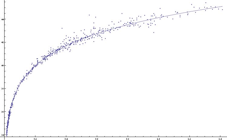
enter image description here

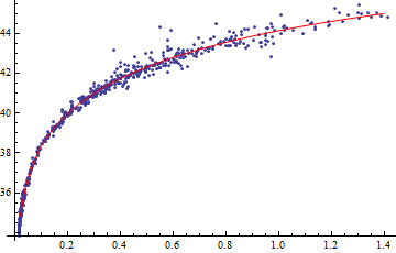
The reality is that the fit is complex

enter image description here

I Have some problems making the fit

  1. Even I put conditions over the parameters $a,b,c$ the fitted model is complex. I tried to put as condition that the whole term inside $\log$ should be positive, but it does not work.
  2. I want to make confidence regions on this fit using

     band1SN[z_] = fit["MeanPredictionBands", ConfidenceLevel -> 0.68]; 
     band2SN[z_] = fit["MeanPredictionBands", ConfidenceLevel -> 0.95];
    

but Mathematica does not make it, an error related with the fact of assuming a constrained model appears. Of course, if the fit is complex, the confidence regions could not be calculated. I appreciate your help.

$\endgroup$

3 Answers 3

2
$\begingroup$

Took another look at this. I don't really have in answer but this may help if anyone want to play with it:

    data = #[[{2, 3}]] & /@ Import["Cat3_0mod.txt", "Table"]

Break the integral into parts with different assumptions and assemble as a Piecewise function: ( results for assumptions -b^2 + 4 a c > 0 and -b^2 + 4 a c <0 are the same if we make the Abs substitution shown )

g3[z_] = Simplify[
      5 Log[10, (1 + z) Integrate[1/(a + b x + c x^2), {x, 0, z}]] + 25, 
      Assumptions -> {z > 0, -b^2 + 4 a c > 0}] /. -b^2 + 4 a c -> Abs[-b^2 + 4 a c]
g1[z_] = Simplify[
     5 Log[10, (1 + z) Integrate[
     1/(a + b x + (b^2/4/a) x^2), {x, 0, z}]] + 25, 
     Assumptions -> {z > 0, a > 0, b > 0, c > 0}]
g0[z_] = Simplify[
     5 Log[10, (1 + z) Integrate[1/(a + b x), {x, 0, z}]] + 25, 
     Assumptions -> {z > 0, a > 0, b > 0}]
g[z_] = Piecewise[ {
   { g0[z] , c == 0} , 
   {g1[z] , -b^2 + 4 a c == 0 }, {g3[z], True}}]

Now do a fit with constraints (this still needs a good inital guess)

   fit = NonlinearModelFit[data, {g[z], {a > 0, b > 0, c >= 0}},
        {{a, 0.0002}, {b, 0.0001}, {c, 0.0001}}, z]

Now take the result an plug it back in as a start point for an unconstrained fit:

   {a0, b0, c0} = {a, b, c} /. fit["BestFitParameters"]
   fit = NonlinearModelFit[data, g[z], {{a, a0}, {b, b0}, {c, c0}}, z]

This last fit finishes quickly with no warnings..

   fit["BestFitParameters"]

{0.000233781, 0.0000547078, 0.000137895}

   Show[{ListPlot[data], Plot[fit[z], {z, 0, 1.4}, PlotStyle -> Red]}, 
     PlotRange -> All]

enter image description here

Unfortunately after all that

  fit["MeanPredictionBands", ConfidenceLevel -> .99]

still gives an error:

"The function value ... is not a number at {a,b,c} = {0.000233781,0.0000547078,0.000137895}

Note the "offending" parameter set is close to the best fit set (It is actually slightly different but not so much so that the sign of b^2-4 a c changes) so I have no idea whats going on there.

$\endgroup$
0
$\begingroup$

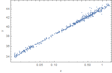
I think your model might be unnecessarily complex. Consider taking the logs of both the dependent and independent variables:

ListLogLogPlot[fitSN, Frame -> True, FrameLabel -> {"z", "y"}]

Data on a log log scale

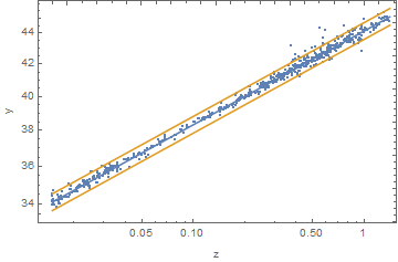
A simple linear model looks like a good candidate model (shown with 95% single prediction intervals):

lm = LinearModelFit[Log[fitSN], z, z];
lm["BestFitParameters"]
(* {3.787583704711951,0.061443756024911325} *)

spb = lm["SinglePredictionBands", ConfidenceLevel -> .95] /. z -> Log[z];
{zmin, zmax} = MinMax[fitSN[[All, 1]]];
Show[ListLogLogPlot[fitSN, Frame -> True, FrameLabel -> {"z", "y"}],
 LogLogPlot[{Exp[lm[Log[z]]], Exp[spb]},
  {z, zmin, zmax}]]

Data and fit on log scale

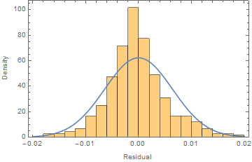
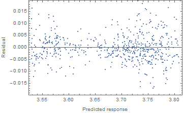
The residual plots don't look great (meaning the assumptions of normality and constant variance) but are much better than what has been proposed by the original model:

ListPlot[Transpose[{lm["PredictedResponse"], lm["FitResiduals"]}],
 Frame -> True, FrameLabel -> {"Predicted response", "Residual"}]
Show[Histogram[lm["FitResiduals"], Automatic, "PDF", Frame -> True,
  FrameLabel -> {"Residual", "Density"}],
 Plot[PDF[
   NormalDistribution[0, StandardDeviation[lm["FitResiduals"]]], x],
  {x, -0.02, 0.02}]]

Histogram of residuals Predicted vs residual

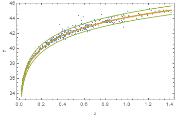
Finally, below is the fitted curve on the original scale:

Show[ListPlot[fitSN], Plot[{Exp[lm[Log[z]]], Exp[mpb], Exp[spb]},
  {z, Min[fitSN[[All, 1]]], Max[fitSN[[All, 1]]]}], Frame -> True,
 FrameLabel -> {"z", "y"}]

Fit and data on original scale

Update

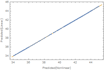
Using all of the work that @george2079 has down in his answer, the linear fit can be compared to the nonlinear fit.

(* Linear fit *)
lm = LinearModelFit[Log[data], z, z]
(* Nonlinear fit *)
fit = NonlinearModelFit[data, g[z], {{a, a0}, {b, b0}, {c, c0}}, z]

{ymin, ymax} = MinMax[data[[All, 2]]]
ListPlot[{Transpose[{fit["PredictedResponse"], Exp[lm["PredictedResponse"]]}],
  {{ymin, ymin}, {ymax, ymax}}}, Joined -> {False, True}, PlotRange -> All,
  Frame -> True, FrameLabel -> {"Predicted(Nonlinear)", "Predicted(Linear)"}]

Nonlinear vs linear fit

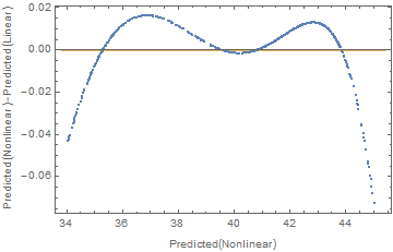
We can look at more detail using the differences in the fit vs the nonlinear fit:

ListPlot[{Transpose[{fit["PredictedResponse"],
    fit["PredictedResponse"] - Exp[lm["PredictedResponse"]]}],
  {{ymin, 0}, {ymax, 0}}}, Joined -> {False, True}, PlotRange -> All, Frame -> True,
 FrameLabel -> {"Predicted(Nonlinear)", "Predicted(Nonlinear)-Predicted(Linear)"}]

Prediction differences vs nonlinear prediction

So we see that the linear fit is generally within plus-or-minus 0.02 of the nonlinear fit. (As to whether the fits are essentially/practically identical is a subject matter call and not a statistical decision.)

$\endgroup$
0
$\begingroup$

My previous answer dealt with an attempt to be convincing that a linear fit (using the logs of both dependent and independent variables) is possibly a better approach. Here I attempt to answer the original question.

@george2079 did all of the work in his answer. All we have to do is remove the Abs function from the definition of g3 and use good starting values:

fit = NonlinearModelFit[data, 
   25 + (5 Log[-((2 (1 + z) (ArcTan[b/Sqrt[-b^2 + 4 a c]] - ArcTan[(b + 2 c z)/Sqrt[-b^2 + 4 a c]]))/Sqrt[-b^2 + 4 a c])])/Log[10],
   {{a, 0.000234}, {b, 0.0000547}, {c, 0.000138}}, z];
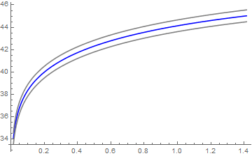
Plot[{fit[z], Evaluate[fit["SinglePredictionBands", ConfidenceLevel -> 0.95]]},
 {z, Min[data[[All, 1]]], Max[data[[All, 1]]]},
 PlotStyle -> {Blue, Gray, Gray}]

Single prediction confidence bands and prediction

I've used "SinglePredictionBands" rather than "MeanPredictionBands" because the mean prediction bands are so close to the predicted curve that they are hard to see.

I believe the issue that causes the problem is that when using Abs the algorithm for finding the prediction bands (probably the Delta Method) takes the derivative of the function with respect to a, b, and c and can't handle the derivative of Abs.

In short, it pays to have really good starting values. Or stated another way: It's always good to know the answer ahead of time.

$\endgroup$

Your Answer

By clicking “Post Your Answer”, you agree to our terms of service and acknowledge you have read our privacy policy.

Not the answer you're looking for? Browse other questions tagged or ask your own question.