Any Mathematica techniques to calculate time takes to reach the equilibrium of a PDE solution

Question

I am solving this PDE numerically (dimensions: spatial variable x and time t). I know how to solve my problem numerically (for a given range of time). The solution reaches its equilibrium after a certain time depending on other parameters of the problem.

ClearAll[uind, x, t];

Du = 1;

alpha = 4;

T = 100;

pde = D[uind[t, x], t] == Du*D[uind[t, x], x, x]-D[uind[t,x],x]-alpha;

bc = {uind[t, 0]== 3, (D[uind[t, x], x] /. x -> 1) == 0};

ic = uind[0, x] == 3;

usol = NDSolve[{pde, ic, bc}, uind, {t, 0, T}, {x, 0, 1}]

Plot3D[{Evaluate[uind[t, x]] /. usol}, {t, 0, T}, {x, 0, 1}, 
 PlotRange -> All, AxesLabel -> {"t", "x", "Sol"}]

I need to calculate the time it takes to reach the equilibrium. Are there any standard Mathematica techniques for that? Any examples in Mathematica are appreciated.

I found this solution, but it does not help me because it is an ODE.

How to use NDSolve to track equilibrium?

Answer 1

Here's a way based on this answer to monitor the time integration and compare a step with the previous step. Integration stops when two steps do not change much compare to the change in time. I used the error norm used by NDSolve (see this and this tutorial), since norm < 1 is the bound on the local error of an integration step. One can substitute one's own custom norm function, but beware of asking for more precision than is being asked of the integration method.

The setup (now) in the OP:

ClearAll[uind, x, t];
Du = 1;
alpha = 4;
T = 100;
pde = D[uind[t, x], t] == 
   Du*D[uind[t, x], x, x] - D[uind[t, x], x] - alpha;
bc = {uind[t, 0] == 3, (D[uind[t, x], x] /. x -> 1) == 0};
ic = uind[0, x] == 3;    

We get data about the NDSolve call when the time integration is initialized. These are documented functions, and relevant details can be found in the plugin tutorial as well as in the tutorials linked above.

Internal`InheritedBlock[{NDSolve`InitializeMethod},
 (* Initialize based on the NDSolve call *)
 Unprotect@NDSolve`InitializeMethod;
 call : NDSolve`InitializeMethod[_, _, sd_, _, state_, ___] /; 
    ! TrueQ[$in] := Block[{$in = True},
   norm = state@"Norm"; (* an NDSolve`ScaledVectorNorm *)
   tlast = NDSolve`SolutionDataComponent[sd, "T"];
   ulast = NDSolve`SolutionDataComponent[sd, "X"];
   call];
 Protect@NDSolve`InitializeMethod;
 
 usol = NDSolve[{
    pde, ic, bc,
    WhenEvent[  (* the equilibrium event *)
     If[t != tlast,(* no event on first step *)
       next = uind[t, x];
       dt = t - tlast;
       du = next - ulast;
       normdu = norm[du/dt, ulast];
       ulast = next;
       tlast = t;
       normdu,
       ulast = uind[t, x];
       1 (* No event *)
       ] < 1,
     {(* I don't like to use Print[] and yet here it is *)
      Print["Reached equilibrium at t = ", t]; 
      "StopIntegration"},
     "LocationMethod" -> "StepEnd"
     ]
    },
   uind, {t, 0, T}, {x, 0, 1}, MaxStepSize -> 1,
   Method -> {"MethodOfLines", "DiscretizedMonitorVariables" -> True}
   ]
 ]

If you don't want to stop the integration at the equilbrium, then replace "StopIntegration" with Nothing. And the event will do nothing. :) (Actually the event action becomes {}, which represents no actions to be taken.)

Update

I'd forgotten how to get the list of values of u[t, x], and, in fact, I had only a vague memory that sometimes you can get an InterpolatingFunction as in the original answer and sometimes a list. Today, I accidentally found "DiscretizedMonitorVariables" -> True in The Method of Lines looking up something else. The above code is more general — it applies to PDEs of any spatial dimension — and it is faster, since it bypasses the construction of an InterpolatingFunction at each step.

---

Old code

The original answer had

next = uind[t, "ValuesOnGrid"]
ulast = uind[t, "ValuesOnGrid"]

with "ValuesOnGrid" instead of x, which replaced it in the update. The following warning applies to using "ValuesOnGrid":

Caveat: I've done this equilibrium detection for a two-dimensional spatial grid, and it needs some tweaking. Normally, when processed inside a WhenEvent, uind[t, x,...] is replaced by ifn[x,...] where ifn is the interpolation at the current time step of uind over the spatial grid. NDSolve does a syntax analysis before going to work, and it requires that uind[..] have the correct number of arguments. So uind[t, "ValuesOnGrid"] does not work if there are two spatial variables. The FEM method works differently than the method of lines, I think, but I don't have time to follow up on that.

Answer 2

btw, you showed no ic, so I made one up.

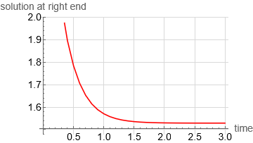
One way to show when equilibrium is reached, since the right side is free (from BC), is to to see when the solution at the right side stops changing. Like this

ClearAll[uind, x, t];

Du = 1;
alpha = 4;
T = 3;
pde = D[uind[t, x], t] == Du*D[uind[t, x], x, x] - D[uind[t, x], x] - alpha;
bc = {uind[t, 0] == 3, (D[uind[t, x], x] /. x -> 1) == 0};
ic = uind[0, x] == 3;
usol = First@NDSolve[{pde, ic, bc}, uind, {t, 0, T}, {x, 0, 1}]

Now make a plot of the value of the solution at the right BC vs. time. When this stops changing, that is where equilibrium is reached

lst = First@Last@Reap@
  Do[Sow[{currentTime, Evaluate[uind[currentTime, 1]] /. usol}], 
      {currentTime, 0.1, 3,0.1}]

and now plot it

ListLinePlot[lst, AxesLabel -> {"time", "solution at right end"}, 
 BaseStyle -> 14, GridLines -> Automatic, GridLinesStyle -> LightGray,
  PlotStyle -> Red]

We see at around 2.5 seconds the solution no longer changes.

How do this automatically? Well, you could use calculus. Take the slope of the above line numerically (data is above), or use a Fit to obtain an actual function that represents the line shape, and when the change in slope (second derivative) gets close to zero, then that is where the equilibrium is reached. I leave this part as an exercise ;).

The above works in this special PDE case only, because you have the right end free. Other BC's cases and other PDE type would require different approach. Ofcourse, if the analytical solution is available that would be much easier to do, but DSolve could not solve this.

Answer 3

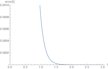
Similar to @Nasser's answer one could define an error function which compares the solutions u[t,x] for different times t:

Du = 1;
alpha = 4;
T = 3;
pde = D[uind[t, x], t] ==Du*D[uind[t, x], x, x] - D[uind[t, x], x] - alpha;
bc = {uind[t, 0] == 3, (D[uind[t, x], x] /. x -> 1) == 0};
ic = uind[0, x] == 3;
U = NDSolveValue[{pde, ic, bc}, uind, {t, 0, T}, {x, 0, 1}]

Assuming that U[T,x] shows the steady state solution, define the error function as follows

error[t_?NumericQ] := NIntegrate[(U[t, x] - U[T, x])^2 , {x, 0, 1}]
Plot[error[t], {t, 0, T}, AxesLabel -> {t, "error[t]"},PlotRange -> {0, .001}] (* takes some time*)

This approach works quite general, it only assumes an existing steady state solution.

Answer 4

Here is another method that is more general in one way and less in another. It uses the values of the time derivative as the measure of when equilibrium has been reached. I approximated the derivative in my other answer, but since the derivative is computed at each step by NDSolve anyway, it makes sense to try to use it. OTOH, it uses the MonitorMethod (see below), which does not work with multistep time-integration methods such the default LSODA.

The OP's example follows. It gives an error because, if there is a way with this method to stop the integration without causing NDSolve to give an error, it is undocumented and I couldn't guess it. The feature of the MonitorMethod is that you can pass a "monitor function" to be called at each step (with access to any of the NDSolve state data). Here I tweaked it so that if the function returns False or $Failed, integration is stopped.

Clear[norm];
mf = Function[{ (* monitor function *)
     h,         (*  next step size (UNUSED) *)
     sd,        (*  SolutionData structure *)
     state,     (*  StateData object *)
     meth},     (*  MethodObject data structure (UNUSED) *)
   If[norm[ (* scaled norm of time-derivative X' relative to X *)
      NDSolve`SolutionDataComponent[sd, "X'"],
      NDSolve`SolutionDataComponent[sd, "X"]
      ] < 1,
    Print["Reached equilibrium at t = ", 
     NDSolve`SolutionDataComponent[sd, "T"]];
    $Failed,
    True, True]];

usol = NDSolve[{pde, ic, bc}, uind, {t, 0, T}, {x, 0, 1}, 
  MaxStepSize -> 1, (* not necessary *)
  Method -> {MonitorMethod,
    "MonitorFunction" -> mf,
    "SaveNormAs" :> norm}]

Note: The step size was restricted because the step size quickly increases to 10. Without the restriction, it overshoots the time at which we are nearly at equilibrium by a bit. If you just want to ensure that equilibrium has been reached, then there is no point in including it.

MonitorMethod:

The MonitorMethod invokes a submethod, but only certain ones are allowed. The documentation does not specify the disallowed methods, but the default Automatic time-integration method, LDSODA, turns out to be one them. Consequently, Automatic defaults to something else here, which I chose to be "StiffnessSwitching". The method may be set with the Method suboption of MonitorMethod.

Other options include "SaveNormAs", which allows the user to save the norm used by NDSolve in an external variable, and "MonitorFunction", which sets the function to be called at each step. The norm is constructed by NDSolve from the PrecisionGoal and AccuracyGoal. The norm is scaled so that norm < 1 indicates an error that is negligible. That criterion is used in mf[] above to detect when the derivative is close enough to zero. The arguments of the monitor function are mf[step_size, SolutionData, StateData, MethodObject]. To change them, change the call to mf[] found in the MonitorMethod[..]["Step"[..]] function.

MonitorMethod // ClearAll;

MonitorMethod // Options = {Method -> Automatic, 
   "MonitorFunction" -> 
    Function[{h, sd, state, meth}, Print[{"H" -> h, "SD" -> sd}]],
   "SaveNormAs" -> Automatic};

MonitorMethod /: 
  NDSolve`InitializeMethod[MonitorMethod, stepmode_, sd_, rhs_, 
   state_, OptionsPattern[MonitorMethod]] := 
  Module[{submethod, mf, norm},
   mf = OptionValue["MonitorFunction"];
   submethod = OptionValue[Method];
   If[submethod === Automatic, submethod = "StiffnessSwitching"];
   submethod = 
    NDSolve`InitializeSubmethod[MonitorMethod, submethod, stepmode, 
     sd, rhs, state];
   norm = OptionValue[Automatic, Automatic, "SaveNormAs", Hold];
   norm /. {
     Hold[Automatic] :> {},
     Hold[nf_] :> (nf = state@"Norm")}; (* get the norm for the user *)
   MonitorMethod[submethod, mf]];

MonitorMethod[submethod_, mf_]["Step"[f_, h_, sd_, state_]] := 
  Module[{res},
   res = NDSolve`InvokeMethod[submethod, f, h, sd, state];
   If[Head[res] === NDSolve`InvokeMethod,
    Return[$Failed]];(* submethod not valid for monitoring *)
   (* call monitor function; stop integration if indicated *)
   If[! FreeQ[mf[h, sd, state, submethod], $Failed | False],
    (* mf indicates stopping *)
    Return[{0, $Failed, MonitorMethod[res[[-1]], mf]}; 
     "StopIntegration"](* causes error *)
    ];
   If[SameQ[res[[-1]], submethod],
    res[[-1]] = Null,
    res[[-1]] = MonitorMethod[res[[-1]], mf]];
   res];

MonitorMethod[___]["StepInput"] = {"Function"[All], "H", 
   "SolutionData", "StateData"};
MonitorMethod[___]["StepOutput"] = {"H", "SD", "MethodObject"};
MonitorMethod[submethod_, ___][prop_] := submethod[prop];

Other uses of MonitorMethod: (199228), (210480)