Couple a PDE and ODE in NDSolve

Question

I would like to solve an example of non-stationary heat transfer with a coupled PDE and ODE. Let's assume that we have 1 dimensional bar of length $L$ with uniform initial temperature. The right end is isolated (no heat flux), and the left end is attached to a (small) isolated reservoir of hot water. The water in the reservoir is well mixed, and we assume it has 0 spatial dimensions. On the boundary between the reservoir and the bar, heat is exchanged by convection, with a known constant coefficient. After enough time has passed, we get uniform temperature in the bar and reservoir, somewhere between both initial temperatures.

Question: How to solve this example with NDSolve command or some similar elegant piece of code?

I have a problem with coupling a PDE ($T[x,t]$) that describes heat transfer inside the bar, and the ODE ($T0[t]$) that describes cooling of the reservoir. It seems that NDSolve can't handle two equations with different number of variables. This is my solution so far, where I solve both equations over the whole domain, but I omit the diffusion term for the reservoir. I think qualitatively the temperature evolution in the bar is appropriate, but the values are wrong.

L = 1.; (* length of domain *)
end = 20.; (* end time *)
k = 2; (* convection coefficient *)
m0 = 100.; (* mass of reservoir *)
Tinit = 0. ;(* initial temperature of the bar *)
T0init = 100.; (* initial temperature of the fluid *)

(* Tsol ... temperature in the bar, T0sol ... temperature on the boundary *)
(* Constants,such as heat conduction coefficient inside the bar, cross-section,etc are omitted for simplicity (assumed to be 1).*)
{Tsol, T0sol} =
NDSolveValue[{
  D[T[t, x], t] - D[T[t, x], x, x] == NeumannValue[-k (T0[t, x] - T[t, x]), x == 0] + NeumannValue[0., x == L]
   , m0*D[T0[t, x], t] == NeumannValue[k (T0[t, x] - T[t, x]), x == 0]
   , T[0, x] == Tinit
   , T0[0, x] == T0init
   }, {T, T0}
  , {t, 0, end}
  , {x, 0, L}
  , Method -> {"MethodOfLines", "SpatialDiscretization" -> "FiniteElement"}
  ]

Manipulate[
 Plot[{Tsol[t, x], T0sol[t, x]}, {x, 0, L}
, PlotRange -> {Automatic, {-1, 110}}
, AxesLabel -> {"x", "Temperature"}
, Epilog -> {Red, PointSize[0.015], Point[{0, T0sol[t, 0]}]}
, PlotLegends -> {"bar", "reservoir"}]
, {t, 0, end}]

Bonus question: How can I extend the solution for another dimension? For example, we have a rectangular domain (the bar), isolated on the right side, with fixed temperature on top and bottom and 1D fluid flow on the left side (advection equation), where heat is exchanged by convection.

Answer 1

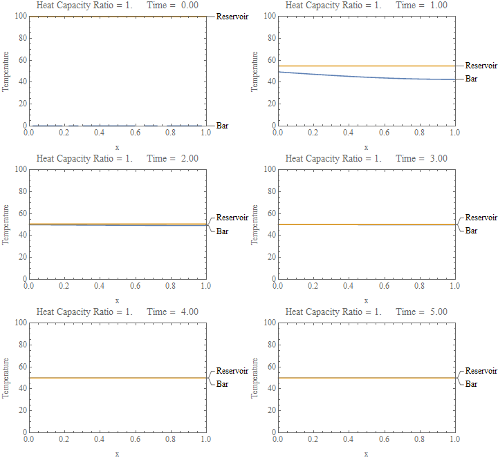
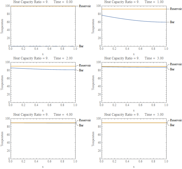
Modified Newton Cooling Law implementation and reduced FEA cell length

Clear["Global`*"]

len = 1;(*length of domain*)
end = 5;(*end time*)
h = 2;(*convection coefficient*)
cpmR = 9;(*heat capacity/mass ratio*)
Tinit = 0;(*initial temperature of the bar*)
T0init = 100;(*initial temperature of the fluid*)

(*Tsol=temperature in the bar,T0sol=temperature on the boundary*)
(*Constants,such as heat conduction coefficient inside the
bar,cross-section,etc are omitted for simplicity (assumed to be 1)*)

{Tsol, T0sol} = NDSolveValue[{
    D[T[t, x], t] - D[T[t, x], x, x] == 
    NeumannValue[h (T[t, x] - T0[t, x]), x == 0] + NeumannValue[0, x == len],
    cpmR D[T0[t, x], t] == -h (T0[t, x] - T[t, x]),
   T[0, x] == Tinit, T0[0, x] == T0init},
  {T, T0}, {t, 0, end}, {x, 0, len},
  Method -> {"MethodOfLines", 
    "SpatialDiscretization" -> {"FiniteElement", 
      "MeshOptions" -> {"MaxCellMeasure" -> {"Length" -> 1*^-4}}}}];

result = Table[Plot[{Tsol[t, x], T0sol[t, 0]}, {x, 0, len},
    PlotRange -> {{0, 1}, {0, T0init}}, 
    FrameLabel -> {"x", "Temperature"}, 
    PlotLabels -> {"Bar", "Reservoir"},
    PlotLabel -> Row@{"Heat Capacity/Mass Ratio = ", N[cpmR], "     ", 
                      "Time = ", PaddedForm[N[t, 3], {3, 2}]},
    BaseStyle -> {FontFamily -> Times, FontSize -> 12}, Frame -> True],
   {t, 0, end, end/100}];
ListAnimate[result]

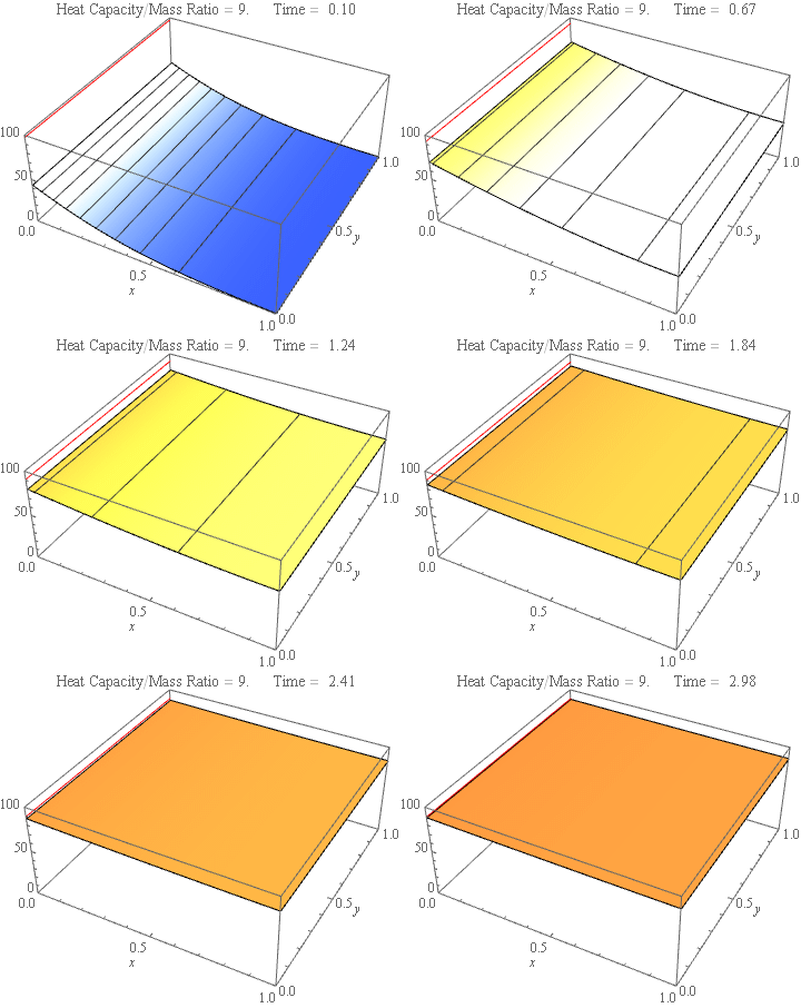
2D Answer:

Clear["Global`*"]

len = 1;(*length of domain*)
wid = 1;(*width of domain*)

end = 3;(*end time*)

h = 2;(*convection coefficient*)
cpmR = 9;(*heat capacity/mass ratio*)

Tinit = 0;(*initial temperature of the bar*)
T0init = 100;(*initial temperature of the fluid*)

Note: Constants, such as thermal conductivity, heat capacity, mass, cross-section, etc are all omitted for simplicity (assumed to be 1)

{Tsol2D, T0sol2D} = NDSolveValue[{
    D[T[t, x, y], t] - (D[T[t, x, y], x, x] + D[T[t, x, y], y, y]) == 
     NeumannValue[-h (T[t, x, y] - T0[t, x, y]), x == 0] + 
      NeumannValue[0, x == len],
    cpmR D[T0[t, x, y], t] == -h (T0[t, x, y] - T[t, x, y]),
    T[0, x, y] == Tinit, T0[0, x, y] == T0init},
   {T, T0}, {t, 0, end}, {x, 0, len}, {y, 0, wid},
   Method -> {"MethodOfLines", "SpatialDiscretization" -> {"FiniteElement"}}];

result2D = 
  Table[Show[
    Plot3D[Tsol2D[t, x, y], {x, 0, len}, {y, 0, wid}, 
     PlotRange -> {{0, len}, {0, wid}, {0, T0init}},
     ColorFunction -> Function[{x, y, z}, ColorData["TemperatureMap"][z/T0init]], 
     ColorFunctionScaling -> False,
     MeshFunctions -> {#3 &}, Mesh -> {Range[5, T0init, 5]}, 
     AxesLabel -> Automatic, 
     PlotLabel ->  Row@{"Heat Capacity/Mass Ratio = ", N[cpmR], "     ", 
                        "Time = ", PaddedForm[N[t, 3], {3, 2}]},
     BaseStyle -> {FontFamily -> Times, FontSize -> 12}], 
    Graphics3D[{Red, 
      Line[{{0, 0, T0sol2D[t, 0, 0]}, {0, 1, T0sol2D[t, 0, 0]}}]}]],
   {t, 1/10, end, end/100}];
ListAnimate[result2D, AnimationRate -> 3]