2
$\begingroup$

Context

The following transient problem is the reciprocating (i.e., fully reversing) flow of a fluid $0<x<L, 0<y<d$ over a thick heated block $0<x<L, -e<y<0$ until the system reaches a cyclic steady-state (i.e., the system temperature oscillates around a mean when this point is reached). The given code simulates the system for a fluid velocity boundary condition $u=3*\sin(2*\pi*1*t)$, i.e., a frequency of $1Hz$ and a heat flux input of $5000 W/m^2$. tflow refers to the total time till which the flow oscillation occurs and t0 is the time-step. The code uses the flow solver developed by Alex Trounev and described in this page and as answer to one of my earlier question here.

Code

Needs["NDSolve`FEM`"]
{f = 2;
 L = 0.040, d = 0.003, e = 0.005, kf = 0.026499, ks = 16, 
 rho = 1.1492, rhos = 7860, mu = 18.923*10^-6, cp = 1.0069*10^3, 
 cps = 502.4}; u0 = 3; nu = mu/rho; om = 2 Pi f;
tflow = 1000;
t0 = .1;
NV = 2 f tflow;
nn = Round[NV \[Pi]/(om t0)]
Ti = 307; q = 5000/Ti;

reg1 = ImplicitRegion[0 <= x <= L && 0 <= y <= d, {x, y}]; reg2 = 
 ImplicitRegion[0 <= x <= L && -e <= y <= d, {x, y}];

mesh = ToElementMesh[FullRegion[2], {{0, L}, {0, d}}];
mesh1 = ToElementMesh[FullRegion[2], {{0, L}, {-e, d}}];
UX[0][x_, y_] := 0;
VY[0][x_, y_] := 0;
P[0][x_, y_] := 0;
Tfs[0][x_, y_] := 307/Ti; appro = 
 With[{k = 2. 10^6}, ArcTan[k #]/Pi + 1/2 &];
ade[y_] := (ks + (kf - ks) appro[y])
rde[y_] := (cps rhos + (cp rho - cps rhos) appro[y]);
eqs = {Inactive[
      Div][({{-\[Mu], 0}, {0, -\[Mu]}}.Inactive[Grad][
        u[x, y], {x, y}]), {x, y}] + D[p[x, y], x] + 
    UX[i - 1][x, y]*D[u[x, y], x] + 
    VY[i - 1][x, y]*D[u[x, y], y] + (u[x, y] - UX[i - 1][x, y])/t0, 
   Inactive[
      Div][({{-\[Mu], 0}, {0, -\[Mu]}}.Inactive[Grad][
        v[x, y], {x, y}]), {x, y}] + D[p[x, y], y] + 
    UX[i - 1][x, y]*D[v[x, y], x] + 
    VY[i - 1][x, y]*D[v[x, y], y] + (v[x, y] - VY[i - 1][x, y])/t0, 
   D[u[x, y], x] + D[v[x, y], y]};
bc[i_] := {DirichletCondition[{u[x, y] == u0*Sin[om*i*t0], 
     v[x, y] == 0}, x == L (1 - Sign[Sin[om*i*t0]])/2 && 0 < y < d], 
   DirichletCondition[{u[x, y] == 0, v[x, y] == 0}, y == 0 || y == d],
    DirichletCondition[p[x, y] == 0, 
    x == L (1 + Sign[Sin[om*i*t0]])/2 && 0 < y < d]};

Monitor[Do[{UX[i], VY[i], P[i]} = 
      NDSolveValue[{eqs == {0, 0, 0} /. \[Mu] -> nu, bc[i]}, {u, v, 
        p}, {x, y} \[Element] mesh, 
       Method -> {"FiniteElement", 
         "InterpolationOrder" -> {u -> 2, v -> 2, p -> 1}}];, {i, 1, 
     nn}], ProgressIndicator[i, {1, nn}]]; // AbsoluteTiming

Monitor[Do[ux = If[y <= 0, 0, UX[i][x, y]];
    vy = If[y <= 0, 0, VY[i][x, y]];
    Tfs[i] = 
     NDSolveValue[{rde[
            y] ((ux*D[T[x, y], x] + 
               vy*D[T[x, y], y]) + (T[x, y] - Tfs[i - 1][x, y])/t0) - 
          Inactive[Div][
           ade[y]*Inactive[Grad][T[x, y], {x, y}], {x, y}] == 
         NeumannValue[q, y == -e], 
        DirichletCondition[{T[x, y] == 1}, 
         x == L (1 - Sign[Sin[om*i*t0]])/2 && 0 <= y <= d]}, 
       T, {x, y} \[Element] mesh1, 
       Method -> {"FiniteElement", 
         "InterpolationOrder" -> {T -> 2}}] // Quiet;, {i, 1, nn}], 
   ProgressIndicator[i, {1, nn}]]; // AbsoluteTiming

ListLinePlot[
  Table[{i t0, Tfs[i][0.5*L, -e/2]*Ti - 273.16}, {i, 0, nn}], 
  AxesLabel -> {"t(s)", "T(in deg. C)"}, PlotRange -> Full]

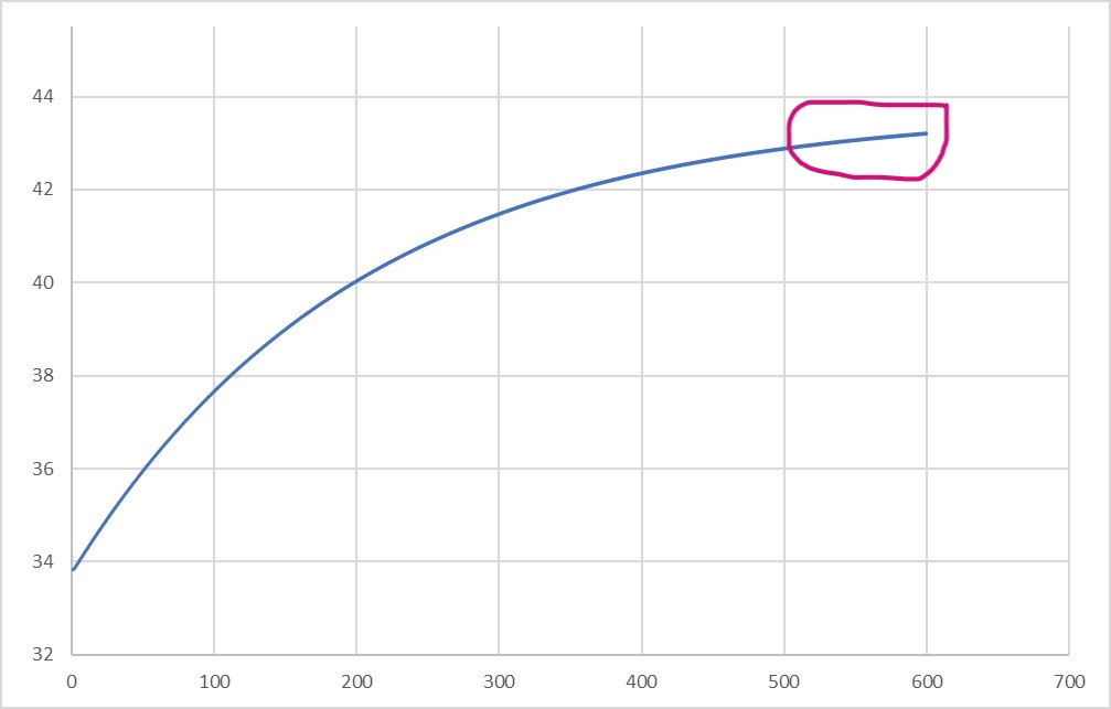
On evaluation, the temperature history of a point (0.5L,-0.5e) in the solid looks like: Time temperature history of point (0.5L,-0.5e) in solid
Question

In essence, the system temperature reaches a cyclic steady state (css) eventually, where it oscillates around a mean value (marked with purple color).

In modelling the system with the approach mentioned here, one has to march through the entire transient phase physically and wait till a css is reached (leading to large simulation times, as the time-step is restricted by the frequency of flow oscillation). My question is, if an alternative approach exists, through which a css can be directly calculated without iterating through the entire flow time? This will be especially useful for high f (which needs even smaller time-steps) and high heat input q (which push reaching css longer) Please note that I am not talking about a steady-state solution, as the flow direction reverses here after each half-cycle.

Some resource

An approach to such direct calculation has been hinted in the Chapter 6-Periodic convection (pp. 259) of the book by Arpaci and Larsen called "Convection heat transfer" and Chapter 6 of the book "Conduction heat transfer" by the same authors. It is named as the method of Complex temperature. A copy of the former can be found here and for the latter here. The method assumes that the solution will oscillate at frequency equal to the imposed excitation frequency. Hence, in this case, the system temperature at css will oscillate with frequency f equal to that imposed in the velocity boundary condition. However, this is an analytical method and the problem at hand is conjugate (i.e., solid-fluid coupled), so its applicability in the present context is doubtful.

Some comparisons

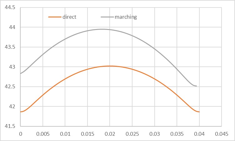
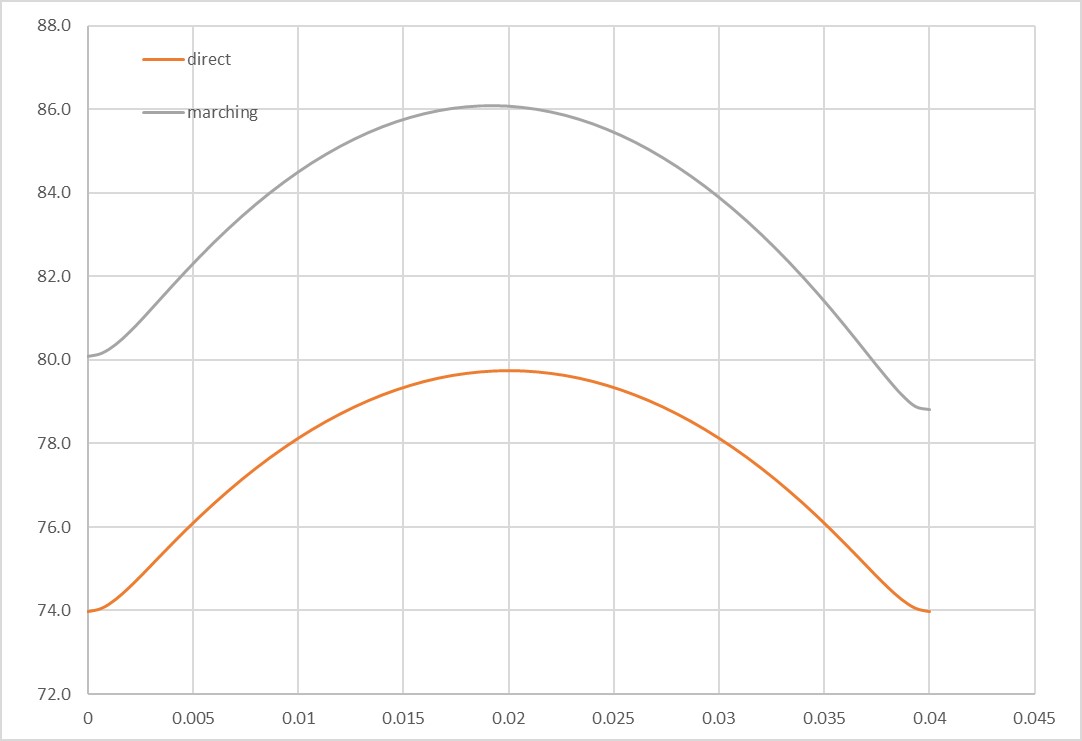
I am naming the original method as marching and the new proposed method by Alex as direct. Using these methods, I ran some comparisons for f=2, u0=3 and q=5000/Ti, 1000/Ti (i.e., different heat inputs). I compared the cyclic average (mean) solid temperature along the line y=-e/2.

For q=5000/Ti

q=5000/Ti

For q=1000/Ti

q=1000/Ti

As evident, there is some considerable difference among the direct and marching solutions. This discrepancy leads to the question as to, which is more accurate in modelling this phenomena?

$\endgroup$
1
  • 1
    $\begingroup$ Please, pay attention that we can include standard deviations in our analysis as follows Tlist = Table[Tfs[i][0.5*L, -e/2]*Ti - 273.16, {i, nn - 49, nn}]; Tmean = Mean[Tlist];dT = StandardDeviation[Tlist] , therefore we have $43.1296\pm 2.69356$ as expected temperature at q=1000/Ti. Also, you computation for Tfs is not complete. May be it goes down after reaching some maximum. $\endgroup$ Commented Dec 16, 2022 at 6:38

1 Answer 1

3
$\begingroup$

Since I am the author of several books and articles in the field of turbulence, I prefer to use statistical methods. For this case, this method can be explained as follows. First, we calculate the hydrodynamic part of the problem. We assume that the phenomenon is periodically repeated. As can be seen from the above graph, the temperature fluctuates relative to the average value. We choose one period and average temperature over that period of time. The simplest algorithm is the following.

Needs["NDSolve`FEM`"]
{f = 2;
 L = 0.040, d = 0.003, e = 0.005, kf = 0.026499, ks = 16, 
 rho = 1.1492, rhos = 7860, mu = 18.923*10^-6, cp = 1.0069*10^3, 
 cps = 502.4}; u0 = 3; nu = mu/rho; om = 2 Pi f;
tflow = 1;
t0 = .01;
NV = 2 f tflow;
nn = Round[NV \[Pi]/(om t0)]
Ti = 307; q = 1000/Ti;

reg1 = ImplicitRegion[0 <= x <= L && 0 <= y <= d, {x, y}]; reg2 = 
 ImplicitRegion[0 <= x <= L && -e <= y <= d, {x, y}];

mesh = ToElementMesh[FullRegion[2], {{0, L}, {0, d}}, 
  MaxCellMeasure -> 10^-7];
mesh1 = ToElementMesh[FullRegion[2], {{0, L}, {-e, d}}, 
  MaxCellMeasure -> 10^-7];
UX[0][x_, y_] := 0;
VY[0][x_, y_] := 0;
P[0][x_, y_] := 0;
Tfs[0][x_, y_] := 307/Ti; appro = 
 With[{k = 2. 10^6}, ArcTan[k #]/Pi + 1/2 &];
ade[y_] := (ks + (kf - ks) appro[y])
rde[y_] := (cps rhos + (cp rho - cps rhos) appro[y]);
eqs = {Inactive[
     Div][({{-\[Mu], 0}, {0, -\[Mu]}} . 
      Inactive[Grad][u[x, y], {x, y}]), {x, y}] + D[p[x, y], x] + 
   UX[i - 1][x, y]*D[u[x, y], x] + 
   VY[i - 1][x, y]*D[u[x, y], y] + (u[x, y] - UX[i - 1][x, y])/t0, 
  Inactive[
     Div][({{-\[Mu], 0}, {0, -\[Mu]}} . 
      Inactive[Grad][v[x, y], {x, y}]), {x, y}] + D[p[x, y], y] + 
   UX[i - 1][x, y]*D[v[x, y], x] + 
   VY[i - 1][x, y]*D[v[x, y], y] + (v[x, y] - VY[i - 1][x, y])/t0, 
  D[u[x, y], x] + D[v[x, y], y]}; 
bc[i_] := {DirichletCondition[{u[x, y] == u0*Sin[om*i*t0], 
    v[x, y] == 0}, x == L (1 - Sign[Sin[om*i*t0]])/2 && 0 < y < d], 
  DirichletCondition[{u[x, y] == 0, v[x, y] == 0}, y == 0 || y == d], 
  DirichletCondition[p[x, y] == 0, 
   x == L (1 + Sign[Sin[om*i*t0]])/2 && 0 < y < d]};

Monitor[Do[{UX[i], VY[i], P[i]} = 
      NDSolveValue[{eqs == {0, 0, 0} /. \[Mu] -> nu, bc[i]}, {u, v, 
        p}, {x, y} \[Element] mesh, 
       Method -> {"FiniteElement", 
         "InterpolationOrder" -> {u -> 2, v -> 2, p -> 1}}];, {i, 1, 
     nn}], ProgressIndicator[i, {1, nn}]]; // AbsoluteTiming

Visualization of the flow for one period

Table[DensityPlot[UX[i][x, y], {x, y} \[Element] mesh, 
  ColorFunction -> "Rainbow", PlotRange -> All, 
  AspectRatio -> Automatic, Frame -> False], {i, nn - 49, nn}]

Figure 1

Monitor[Do[ux = If[y <= 0, 0, UX[i][x, y]]; 
    vy = If[y <= 0, 0, VY[i][x, y]];
    Tfs[i] = 
     NDSolveValue[{rde[y] ((ux*D[T[x, y], x] + vy*D[T[x, y], y])) - 
          Inactive[Div][
           ade[y]*Inactive[Grad][T[x, y], {x, y}], {x, y}] == 
         NeumannValue[q, y == -e], 
        DirichletCondition[{T[x, y] == 1}, 
         x == L (1 - Sign[Sin[om*i*t0]])/2 && 0 <= y <= d]}, 
       T, {x, y} \[Element] mesh1, 
       Method -> {"FiniteElement", 
         "InterpolationOrder" -> {T -> 2}}] // Quiet;, {i, nn - 49, 
     nn}], ProgressIndicator[i, {nn - 49, nn}]]; // AbsoluteTiming

Visualization of the mean temperature Figure 2 Mean temperature in a fixed point

Sum[Tfs[i][0.5*L, -e/2]*Ti - 273.16, {i, nn - 49, nn}]/50

Out[]= 43.1296

From our answer here it should be about 44.165.

$\endgroup$
12
  • $\begingroup$ If I understand correctly, you have calculated the flow field for one second, i.e., two time periods. Then, you have utilized the flow field for one time-period to solve for a steady-state solution of the energy equation ? $\endgroup$
    – Avrana
    Commented Dec 15, 2022 at 10:45
  • $\begingroup$ Yes, it is right. $\endgroup$ Commented Dec 15, 2022 at 15:57
  • $\begingroup$ I have been using the new method suggested by you. It does seem logical to find the css this way. However, I ran some comparative tests among the old and new approaches, the results of which I have added as a new section to the original question. As you will be seeing, there is some considerable difference among the results. This leads to the confusion as to which should be adopted as the correct. Although it does seem, that the direct method is more accurate as it is capable of using a very small time-step and very fine mesh size. $\endgroup$
    – Avrana
    Commented Dec 16, 2022 at 5:18
  • $\begingroup$ Apologies for the late reply. I have been travelling. I am still testing the method for some cases and it seems to be working. Meanwhile, can you kindly point to some references you mentioned in the first line of your answer here, where this method is described more in detail. $\endgroup$
    – Avrana
    Commented Dec 17, 2022 at 6:46
  • 1
    $\begingroup$ It does not matter since $\rho$ is a constant, and we use homogeneous bc as DirichletCondition[p[x, y] == 0, x == L (1 + Sign[Sin[om*i*t0]])/2 && 0 < y < d]. $\endgroup$ Commented Dec 28, 2022 at 8:30

Your Answer

By clicking “Post Your Answer”, you agree to our terms of service and acknowledge you have read our privacy policy.

Not the answer you're looking for? Browse other questions tagged or ask your own question.