4
$\begingroup$

I'm plotting the numerical solution of a differential equations, using the altitude-like level curves as a mesh. It's fine, but I would like to add three specific altitude levels as thick red, green and blue curves, while all other curves stay in the default style. Here's a simple MWE to play with:

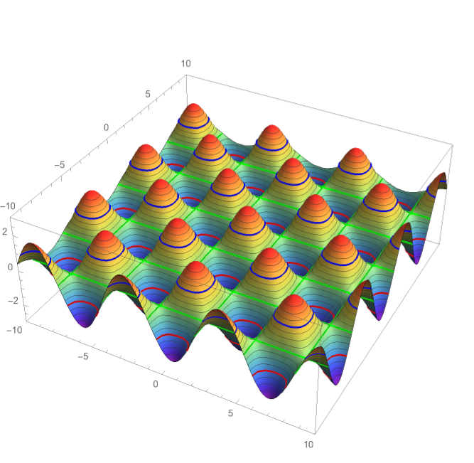
Plot3D[
 Sin[x - y] + Cos[x + y], (* this function is just for the MWE *)
 {x, -10, 10},
 {y, -10, 10},
 PlotPoints -> {30, 30},
 PlotRange -> {{-10, 10}, {-10, 10}, {-3, 3}},
 MeshFunctions -> (#3 &),
 ColorFunction -> "Rainbow",
 ImageSize -> 500,
 Method -> {"RotationControl" -> "Globe"},
 SphericalRegion -> True
 ]

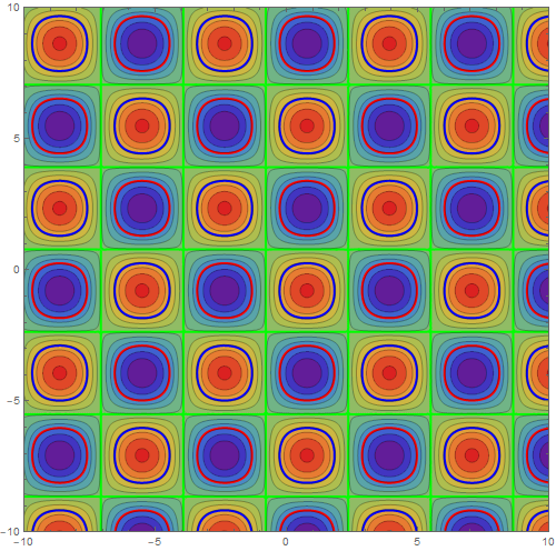
ContourPlot[
 Sin[x - y] + Cos[x + y], (* this function is just for the MWE *)
 {x, -10, 10},
 {y, -10, 10},
 PlotPoints -> {30, 30},
 PlotRange -> {{-10, 10}, {-10, 10}},
 ColorFunction -> "Rainbow",
 ImageSize -> 500
 ]

So I need this:

On both plots, I need to show the level curves for the alitude -1 (in thick red), 0 (in thick green) and +1 (in thick blue), while keeping all other curves as they currently are. These curves should be independent of the particular function that I use in this MWE.

How can I do this?

$\endgroup$
0

3 Answers 3

7
$\begingroup$

You can use multiple mesh functions in a plot, each with its own mesh definitions:

Plot3D[
 Sin[x - y] + Cos[x + y],
 {x, -10, 10},{y, -10, 10},
 PlotPoints -> {30, 30},
 PlotRange -> {{-10, 10}, {-10, 10}, {-3, 3}},
 Mesh -> {
   Range[-5, 5, 0.5] (*"regular" mesh*),
   {(*your own special lines*)
     {-1, Directive[Thick, Red]},
     {0, Directive[Thick, Green]},
     {1, Directive[Thick, Blue]}}
   },
 MeshFunctions -> {(#3 &),(#3&)},
 ColorFunction -> "Rainbow",
 ImageSize -> 500,
 Method -> {"RotationControl" -> "Globe"},
 SphericalRegion -> True
]

Plot3D with desired meshes


It is even easier with ContourPlot, where you can just provide a list of contour values. Generate a list of standard contours with Range, styled by the ContoursStyle option, then Join it with a list of your special contours, hand-styled as you wish them to be.

ContourPlot[
 Sin[x - y] + Cos[x + y], {x, -10, 10}, {y, -10, 10},
 PlotRange -> {{-10, 10}, {-10, 10}},
 PlotPoints -> {30, 30},
 ColorFunction -> "Rainbow",

 (* styling for default contours *)
 ContourStyle -> Opacity[0.3],
 Contours -> 
   Join[
     (* default contours *)
     Range[-5, 5, 0.33],
     (* your own hand-styled ones *)
     {
       {-1, Directive[Opacity[1, Red], Thick]},
       {0, Directive[Opacity[1, Green], Thick]},
       {1, Directive[Opacity[1, Blue], Thick]}
     }
   ],
 ImageSize -> 500
]

contourplot with styled contours

$\endgroup$
6
  • $\begingroup$ Is this also working for the CountourPlot? $\endgroup$
    – Cham
    Commented Dec 7, 2020 at 14:26
  • $\begingroup$ Aaah! Stupid I am! I forgot your MeshFunctions -> {(#3 &),(#3&)}. Now it's working! $\endgroup$
    – Cham
    Commented Dec 7, 2020 at 15:00
  • $\begingroup$ How do you make the default mesh to have style? I would add opacity 50% or gray level. $\endgroup$
    – Cham
    Commented Dec 7, 2020 at 15:29
  • $\begingroup$ YES! It works very nicely now! Woowee, that was a lot of work! Thanks a lot!! $\endgroup$
    – Cham
    Commented Dec 7, 2020 at 17:21
  • $\begingroup$ I just noticed a mismatch in altitude curves on the 2D view. The red, green and blue curves are perfect on the 3D view, but they aren't at their proper location on the 2D view. I don't understand what is going on here, with the Join function: Contours -> Join[ Range[-5, 5, 01/3], { {-1, Directive[Red, Thick]}, {0, Directive[Green, Thick]}, {1, Directive[Blue, Thick]} } ]. The curves are offset by 1 or 2 positions. $\endgroup$
    – Cham
    Commented Dec 7, 2020 at 22:33
5
$\begingroup$

All the methods below add three styled curves, "while all other curves stay in the default style."

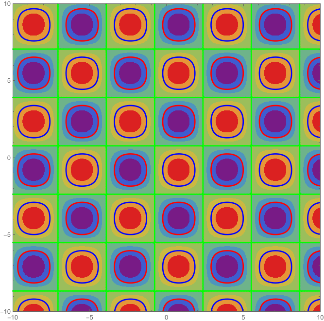
ContourPlot

1. You can use the options MeshFunctions and Mesh to add additional contours:

ContourPlot[Sin[x - y] + Cos[x + y], {x, -10, 10}, {y, -10, 10}, 
 PlotPoints -> {30, 30}, PlotRange -> {{-10, 10}, {-10, 10}}, 
 ColorFunction -> "Rainbow", ImageSize -> 500,
 MeshFunctions -> {Sin[# - #2] + Cos[# + #2] &}, 
 Mesh -> {Thread[{{0., -1., 1.}, 
     Thread[Directive[{Green, Red, Blue}, Thick, Opacity[1]]]}]}]
enter image description here

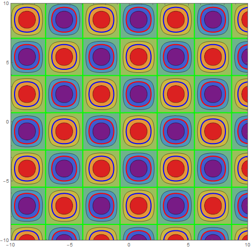
2. Generate the list of contours using FindDivisions and style each contour as you like:

automaticcontours = FindDivisions[{-2, 2}, 10];

styledcontours = {{-1, Directive[Thick, Red]}, 
   {0, Directive[Thick, Green]}, {1, Directive[Thick, Blue]}};

contours = DeleteDuplicatesBy[First]@
   Join[styledcontours, Thread[{automaticcontours, Automatic}]];

ContourPlot[Sin[x - y] + Cos[x + y], {x, -10, 10}, {y, -10, 10}, 
 PlotPoints -> {30, 30}, PlotRange -> {{-10, 10}, {-10, 10}}, 
 ColorFunction -> "Rainbow", ImageSize -> 500, 
 Contours -> contours]
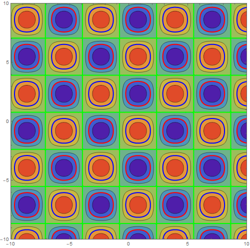
enter image description here

3. Post-process ContourPlot output to restyle selected contours:

cp = ContourPlot[Sin[x - y] + Cos[x + y], {x, -10, 10}, {y, -10, 10}, 
  PlotPoints -> {30, 30}, PlotRange -> {{-10, 10}, {-10, 10}}, 
  ColorFunction -> "Rainbow", ImageSize -> 500];

Replace[cp, {Tooltip[{d___, l__Line}, t : (0. | 1. | -1.)] :> {Thick, Opacity[1], 
    t /. {0. -> Green, -1. -> Red, 1. -> Blue, _ -> {d}},  Tooltip[{l}, t]}}, All]

enter image description here

4. Yet another method is to extract the contours from cp and redo ContourPlot using styled contours:

automaticcontours = Cases[cp, Tooltip[_, t_] :> t, All]
{1.5, 1., 0.5, 0., -0.5, -1., -1.5};
styledcontours = Thread[{{0., -1., 1.}, 
     Thread[Directive[{Green, Red, Blue}, Thick, Opacity[1]]]}];

contours = Join[styledcontours , Complement[automaticcontours, {0., -1., 1.}]];

ContourPlot[Sin[x - y] + Cos[x + y], {x, -10, 10}, {y, -10, 10}, 
 PlotPoints -> {30, 30}, PlotRange -> {{-10, 10}, {-10, 10}}, 
 ColorFunction -> "Rainbow", ImageSize -> 500, 
 Contours -> contours]
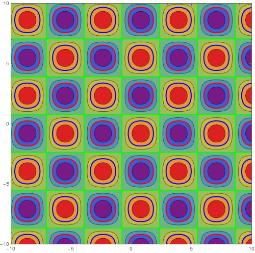
enter image description here

Plot3D

1. Use FindDivisions to generate a mesh list (that matches the automatically generated one) and add your list of styled mesh lines and use the combined list as the setting for Mesh:

automaticmeshlines = Most @ Rest @ FindDivisions[{-2, 2}, 18];

styledmeshlines = {{-1, Directive[Thick, Red]}, {0, 
    Directive[Thick, Green]}, {1, Directive[Thick, Blue]}};

mesh = DeleteDuplicatesBy[First]@
  Join[styledmeshlines, Thread[{automaticmeshlines , Automatic}]];

Plot3D[Sin[x - y] + Cos[x + y], {x, -10, 10}, {y, -10, 10}, 
 PlotPoints -> {30, 30}, PlotRange -> {{-10, 10}, {-10, 10}, {-3, 3}},
 ColorFunction -> "Rainbow", ImageSize -> 500, 
 Method -> {"RotationControl" -> "Globe"}, SphericalRegion -> True,
 MeshFunctions -> {#3 &},
 Mesh -> {mesh}]

enter image description here

2. Add constant functions in the first argument of Plot3D corresponding to the desired levels, set their PlotStyle to Opacity[0] and use the option BoundaryStyle to set the directives for the intersection of the main surface with the added planes:

Plot3D[{ 0., -1., 1., Sin[x - y] + Cos[x + y]}, {x, -10, 10}, {y, -10,
   10}, PlotPoints -> {30, 30}, 
 PlotRange -> {{-10, 10}, {-10, 10}, {-3, 3}}, 
 MeshFunctions -> (#3 &), 
 PlotStyle -> {Opacity[0], Opacity[0], Opacity[0], Automatic}, 
 ColorFunction -> "Rainbow", ImageSize -> 500, 
 BoundaryStyle -> {1 -> None, 2 -> None, 3 -> None, 
   {4, 1} -> Directive[Green, AbsoluteThickness[4], Opacity[1]], 
   {4, 2} -> Directive[Red, AbsoluteThickness[4], Opacity[1]],
   {4, 3} -> Directive[Blue, AbsoluteThickness[4], Opacity[1]]}, 
 Method -> {"RotationControl" -> "Globe"}, SphericalRegion -> True]
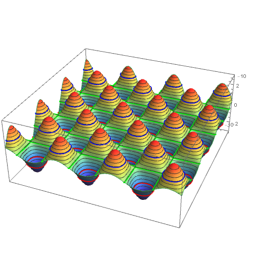
enter image description here

3. Post-process to restyle selected mesh lines:

p3d = Plot3D[Sin[x - y] + Cos[x + y], {x, -10, 10}, {y, -10, 10}, 
  PlotPoints -> {30, 30}, 
  PlotRange -> {{-10, 10}, {-10, 10}, {-3, 3}}, 
  MeshFunctions -> (#3 &), ColorFunction -> "Rainbow", 
  ImageSize -> 500, Method -> {"RotationControl" -> "Globe"}, 
  SphericalRegion -> True];

Normal[p3d] /. Line[x_, ___] :> 
  {Round[x[[1, -1]], 0.1] /. Append[Thread[{0., -1., 1.} -> 
    Thread[Directive[{Green, Red, Blue}, Thick, Opacity[1]]]], _ -> {}],  Line[x]}
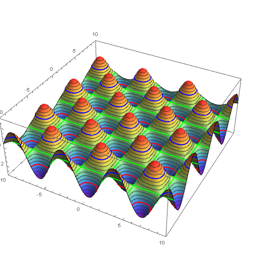
enter image description here

$\endgroup$
3
  • $\begingroup$ The first method appears to be adapted to the specific function given as an example. I need it to be independent of the function, since the real code is about displaying a numerical solution of some differential equation... $\endgroup$
    – Cham
    Commented Dec 7, 2020 at 15:22
  • $\begingroup$ @Cham, in general, you can use the function in the first argument of ContourPlot as the mesh function. That is, use ContourPlot[foo[x,y], ..., MeshFunctions->{foo[#,#2]&},....] or ContourPlot[foo[x,y], ..., MeshFunctions->{Function[{x,y},foo[x,y]]},....] $\endgroup$
    – kglr
    Commented Dec 7, 2020 at 15:40
  • $\begingroup$ Agreed. But since my function is a numerical solution, I don't know how to set it up in there. Using Phi[t,#1, #2]& alone doesn't work. With Evaluate, it doesn't work neither, yet. $\endgroup$
    – Cham
    Commented Dec 7, 2020 at 15:50
5
$\begingroup$

3D

Set the Mesh to

 Mesh -> {{{-1, {Thick, Red}}, {0, {Thick, Green}}, {1, {Thick, 
        Blue}}}}
a = Plot3D[
   Sin[x - y] + 
    Cos[x + y],(*this function is just for the MWE*){x, -10, 
    10}, {y, -10, 10}, PlotPoints -> {30, 30}, 
   PlotRange -> {{-10, 10}, {-10, 10}, {-3, 3}}, 
   MeshFunctions -> (#3 &), ColorFunction -> "Rainbow", 
   ImageSize -> 500, Method -> {"RotationControl" -> "Globe"}, 
   SphericalRegion -> True];
b = Plot3D[Sin[x - y] + Cos[x + y], {x, -10, 10}, {y, -10, 10}, 
   PlotPoints -> {30, 30}, 
   PlotRange -> {{-10, 10}, {-10, 10}, {-3, 3}}, 
   MeshFunctions -> (#3 &), 
   Mesh -> {{{-1, {Thick, Red}}, {0, {Thick, Green}}, {1, {Thick, 
        Blue}}}}, PlotStyle -> None];
Show[a, b]

enter image description here

2D

Set Contours

Contours -> {{-1, {Thick, Red}}, {0, {Thick, Green}}, {1, {Thick, 
       Blue}}}
aa = ContourPlot[
   Sin[x - y] + 
    Cos[x + y],(*this function is just for the MWE*){x, -10, 
    10}, {y, -10, 10}, PlotPoints -> {30, 30}, 
   PlotRange -> {{-10, 10}, {-10, 10}}, ColorFunction -> "Rainbow", 
   ImageSize -> 500];
bb = ContourPlot[Sin[x - y] + Cos[x + y], {x, -10, 10}, {y, -10, 10}, 
   PlotPoints -> {30, 30}, PlotRange -> {{-10, 10}, {-10, 10}}, 
   ImageSize -> 500, ContourShading -> None, 
   Contours -> {{-1, {Thick, Red}}, {0, {Thick, Green}}, {1, {Thick, 
       Blue}}}];
Show[aa, bb]

Or this?

aa = ContourPlot[
   Sin[x - y] + 
    Cos[x + y],(*this function is just for the MWE*){x, -10, 
    10}, {y, -10, 10}, PlotPoints -> {30, 30}, 
   PlotRange -> {{-10, 10}, {-10, 10}}, ColorFunction -> "Rainbow", 
   ImageSize -> 500, MeshFunctions -> (#3 &), Mesh -> None, 
   ContourStyle -> None, ContourShading -> Automatic];
bb = ContourPlot[Sin[x - y] + Cos[x + y], {x, -10, 10}, {y, -10, 10}, 
   PlotPoints -> {30, 30}, PlotRange -> {{-10, 10}, {-10, 10}}, 
   ImageSize -> 500, ContourShading -> None, ContourStyle -> None, 
   MeshFunctions -> (-#3 &), 
   Mesh -> {{{-1, {Thick, Red, Opacity[1]}}, {0, {Thick, Green, 
        Opacity[1]}}, {1, {Thick, Blue, Opacity[1]}}}}];
Show[aa, bb]

enter image description here

$\endgroup$
0

Your Answer

By clicking “Post Your Answer”, you agree to our terms of service and acknowledge you have read our privacy policy.

Not the answer you're looking for? Browse other questions tagged or ask your own question.