4
$\begingroup$

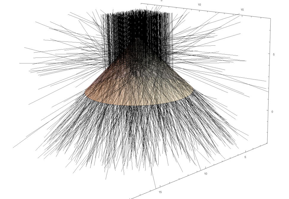
I used Tim Laska's solution here for raytracing, and modelled 10000 photons impinging onto a cone.

shape = Cone[{{7.5, 7.5, 1}, {7.5, 7.5, 6}}, 5]

(* 10 000 photons *) 
data2 = Import[
    "https://raw.githubusercontent.com/Tb8854/overflowquestion/master/\
test", "Data"][[1]];
data2 = ToExpression[data2];

(* plot first 1000 *) 
data = data2[[1 ;; 1000]];
data = Flatten[data[[#]], 2] & /@ Range[Length[data]];
lines = Line[#] & /@ data;
Graphics3D[{lines, {Opacity[0.4], shape}}, 
 PlotRange -> {{2, 18}, {2, 18}, {-3, 8}}, Axes -> True, 
 Boxed -> False]

enter image description here

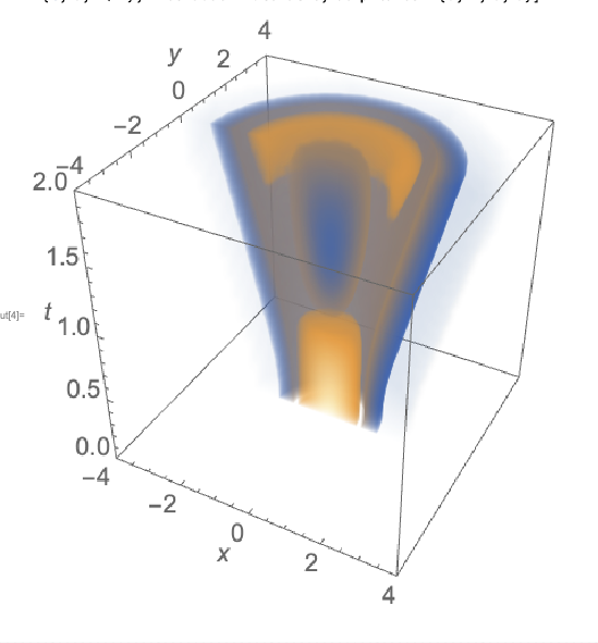
But, I want to see the flux, i.e. the number of rays (i.e. lines) per unit area in the material. Maybe something like this:

enter image description here

Where, if I a higher density of lines the cone, the redder the cone should be. I don't think the rays in the first image effectively show the spreading out of the rays when they enter the cone.


A Poor Solution

I've developed a poor 2D solution, beware - it takes a while (2 minutes). What it does is make slices in the cone, and check if there is an intersection. It works okay.

datastore = ConstantArray[{}, (5)];
points = ConstantArray[{}, {(5), Length[data]}];
(* prevent hitting the edge *) 
positionerror = 0.01;

For[j = 5, j >= 1, j = j - 1,
 Print[j]; 
 number = 0; 
 plane = InfinitePlane[{10, 10, 
    j + positionerror}, {{0, 1, 0}, {1, 0, 0}}];

 Monitor[For[i = 1, i <= Length[data], i++, 
   line = Line[data[[i]]];
   intersection = RegionIntersection[plane, line, shape];
   points[[j, i]] = intersection;
   If[intersection === EmptyRegion[3], 
    Continue[];, 
    number = number + 1;
    ];

   area = Area[Region[RegionIntersection[plane, shape]]];
   datastore[[j]] = {number, area, number/area};

   ], ProgressIndicator[i, {1, Length[data]}]]]


For[i = 2.01, i <= 6, i++, 
  pointsplot = 
   Select[Flatten[points[[2 ;;, ;; , 1]], 2], Length[#] == 3 &];
  pointsplot = Select[pointsplot, #[[3]] == i &];
  pointsplot = pointsplot[[;; , {1, 2}]];

  data = BinCounts[pointsplot, {2, 13, 0.1}, {2, 13, 0.1}];
  data = GaussianFilter[data, 2];
  Print[ListDensityPlot[data, ColorFunction -> "BlueGreenYellow", 
    PlotRange -> All]]
  ];

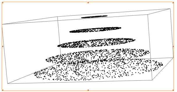
Graphics3D[{points}]

enter image description here enter image description here

But does anyone have any ideas how to maybe represent the flux in 3D?

$\endgroup$
6
  • $\begingroup$ Could you explain your definition of flux? I don't really understand what's going on in the top diagram. There's a related concept in subsurface scattering where rays enter the object from all directions, are attenuated by the material, and you can calculate the average energy going through a small sphere at some point on the interior. $\endgroup$
    – flinty
    Commented Jun 6, 2020 at 20:25
  • $\begingroup$ I want to represent a scalar flux. So the number of rays in an area, i.e. rays/unit area. It could also be the volume. I.e the number of rays in a unit volume. The top diagram is just the rays from the raytracer. So, the rays are coming in and interacting with the cone. Some travel into the cone. I want to effectively represent the spreading out of the rays in the cone. I think this correlates to the picture you describe in subsurface scattering if we assign each ray an energy. $\endgroup$
    – Tomi
    Commented Jun 6, 2020 at 21:27
  • $\begingroup$ What %age of rays enter the cone? Does the cone have a refractive index, opacity, roughness - and a reflectance model etc. ? $\endgroup$
    – flinty
    Commented Jun 6, 2020 at 21:42
  • $\begingroup$ The cone only has a refractive index (n=1.7). However, the cone is a very much simplified shape for the MWE here. Also, in the real simulation the rays come from all directions. $\endgroup$
    – Tomi
    Commented Jun 6, 2020 at 21:45
  • $\begingroup$ The flux for the 3D example: at any given point within the cone, count the number of intersections of an arbitrarily small cube with all rays and divide by the cube's surface area. This gives you an estimate of the flux at that point. This is an extremely expensive calculation with this many rays. I'm having trouble thinking how to speed it up. $\endgroup$
    – flinty
    Commented Jun 6, 2020 at 22:47

1 Answer 1

6
$\begingroup$

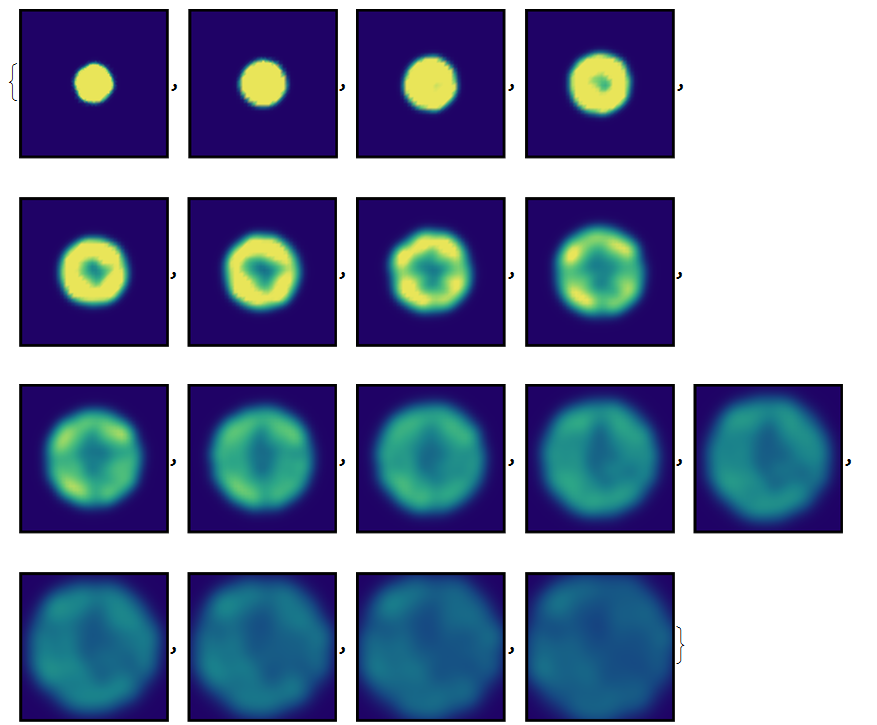
Maybe SmoothDensityHistogram could help smooth out and visualize the flux.

poincarePlane[p_] := 
 Select[Flatten[points[[2 ;;, ;; , 1]], 2], 
   Length[#] == 3 && (Abs[#[[3]] - p] < 0.01) &][[All, {1, 2}]]
Column[SmoothDensityHistogram[poincarePlane[#], 
    ColorFunction -> 
     Function[{z}, ColorData["BlueGreenYellow"][10 z]], 
    ColorFunctionScaling -> False, 
    PlotRange -> RegionBounds[shape][[1 ;; 2]]] & /@ 
  Reverse@{2.01, 3.01, 4.01, 5.01}]

HistogramImages

You could try constructing a 3D model using Image3D as describe by C.E. in this broccoli reconstruction MSE answer here.

Update

I have not tried to optimize Tomi's code, but I increased the number of planes from 5->20.

datastore = ConstantArray[{}, (20)];
points = ConstantArray[{}, {(20), Length[data]}];
(*prevent hitting the edge*)
positionerror = 0.01;

For[j = 20, j >= 1, j = j - 1, Print[j];
 number = 0;
 plane = InfinitePlane[{10, 10, 
    j/4 + positionerror}, {{0, 1, 0}, {1, 0, 0}}];
 Monitor[For[i = 1, i <= Length[data], i++, line = Line[data[[i]]];
   intersection = RegionIntersection[plane, line, shape];
   points[[j, i]] = intersection;
   If[intersection === EmptyRegion[3], Continue[];, 
    number = number + 1;];
   area = Area[Region[RegionIntersection[plane, shape]]];
   datastore[[j]] = {number, area, number/area};], 
  ProgressIndicator[i, {1, Length[data]}]]]

Here are the images at finer z-spacing:

cuts = Table[i + 0.01, {i, 1, 5., 0.25}];
poincarePlane[p_] := 
 Select[Flatten[points[[2 ;;, ;; , 1]], 2], 
   Length[#] == 3 && (Abs[#[[3]] - p] < 0.01) &][[All, {1, 2}]]
imgs = Rasterize@
    SmoothDensityHistogram[poincarePlane[#], 
     ColorFunction -> 
      Function[{z}, ColorData["BlueGreenYellow"][20 z]], 
     ColorFunctionScaling -> False, Background -> Black, 
     PlotRange -> RegionBounds[shape][[1 ;; 2]], ImageSize -> Small, 
     FrameTicks -> None, ImagePadding -> None] & /@ Reverse@cuts

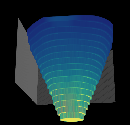
Images at finer z spacing

3D Reconstruction Using Image3D

Using @C.E.'s approach linked above:

imgs = MapThread[SetAlphaChannel, {imgs, Binarize /@ imgs}];
Image3D[imgs, Background -> Black, BoxRatios -> {1, 1, 1}]

Image3D Reconstruction

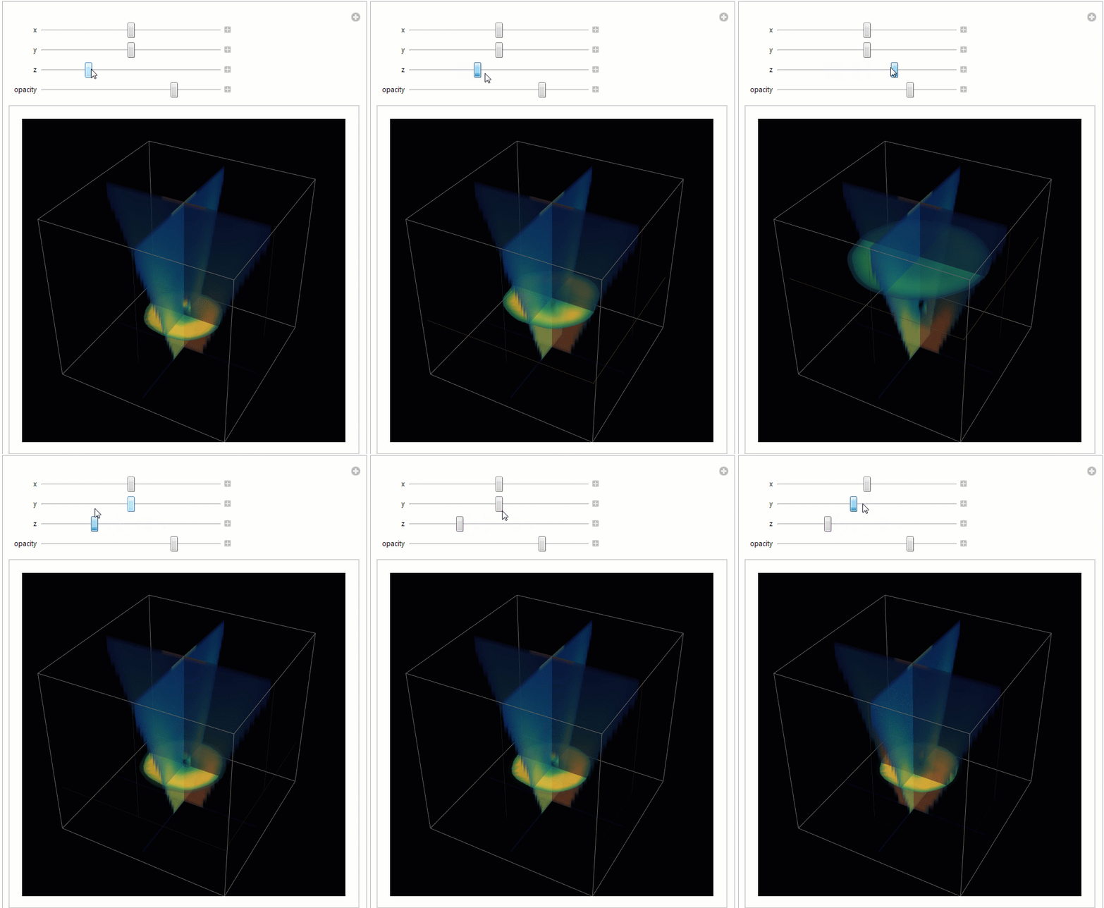
Dynamic Cut Plane Visualization

The Texture shows how to create an efficient dynamic clip planes visualization.

data = Developer`ToPackedArray[Map[ImageData, imgs]];
Manipulate[
 Graphics3D[{Opacity[Dynamic[o]], Texture[data], EdgeForm[None],
   Dynamic[{Polygon[{{x, 0, 0}, {x, 1, 0}, {x, 1, 1}, {x, 0, 1}}, 
      VertexTextureCoordinates -> {{x, 0, 0}, {x, 1, 0}, {x, 1, 
         1}, {x, 0, 1}}], 
     Polygon[{{0, y, 0}, {1, y, 0}, {1, y, 1}, {0, y, 1}}, 
      VertexTextureCoordinates -> {{0, y, 0}, {1, y, 0}, {1, y, 
         1}, {0, y, 1}}],
     Polygon[{{0, 0, 1 z}, {1, 0, 1 z}, {1, 1, 1 z}, {0, 1, 1 z}}, 
      VertexTextureCoordinates -> {{0, 0, 1 z}, {1, 0, 1 z}, {1, 1, 
         1 z}, {0, 1, 1 z}}]}]}, Background -> Black, 
  RotationAction -> "Clip"], {{x, 0.5}, 0, 1}, {{y, 0.5}, 0, 
  1}, {{z, 0.5}, 0, 1}, {{o, 0.75, "opacity"}, 0, 1}, 
 ControlPlacement -> Top]

Dynamic Slicing

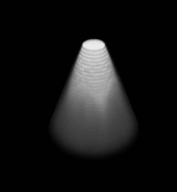
Update to Include Volume Rendering Customization

One may desire finer control over the Opacity to obtain the desired volume rendering. @Jason B's MSE answer here shows a way to achieve this using ListDensityPlot3D.

In this case, I ran @Tomi's work flow on the full dataset on 40 planes overnight and applied the following workflow to generate an Image3D.

cuts = Table[i + 0.01, {i, 1, 5., 0.125}];
pts = Transpose[
   Select[Flatten[points[[2 ;;, ;; , 1]], 2], Length[#] == 3 &]];
poincarePlane[p_] := 
 Select[Flatten[points[[2 ;;, ;; , 1]], 2], 
   Length[#] == 3 && (Abs[#[[3]] - p] < 0.01) &][[All, {1, 2}]]
imgs = Rasterize@
     SmoothDensityHistogram[poincarePlane[#], 
      ColorFunction -> Function[{z}, ColorData["GrayTones"][40 z]], 
      PlotRange -> {{1.5, 13.5}, {1.5, 13.5}}, 
      RegionFunction -> Function[{x, y, z}, z >= 0.001], 
      ColorFunctionScaling -> False, Background -> Black, 
      ImageSize -> Medium, FrameTicks -> None] & /@ Reverse@cuts;
imgs = ColorConvert[ImageCrop[#, 590] & /@ imgs, "Grayscale"];
i3d = Image3D[imgs, Background -> Black, BoxRatios -> {1, 1, 1}, 
  ColorFunction -> "XRay"]

Xray

Now, we can apply @Jason B's workflow to explore different OpacityFunctions.

list = ImageData /@ Image3DSlices[i3d];
Plot[Evaluate[(Exp[# f] - 1)/(E^# - 1) & /@ {1, 4, 8, 12}], {f, 0, 1}]
ListDensityPlot3D[list, 
   OpacityFunction -> Function[f, (Exp[# f] - 1)/(E^# - 1)], 
   ColorFunction -> ColorData["BlueGreenYellow"], 
   RegionFunction -> 
    Function[{x, y, z, f}, ! ((x >= 7.5) && (y <= 7.5))], 
   ImageSize -> 300, Background -> Black, 
   DataRange -> MinMax /@ pts] & /@ {1, 4, 8, 12}

Volume Rendering

$\endgroup$

Your Answer

By clicking “Post Your Answer”, you agree to our terms of service and acknowledge you have read our privacy policy.

Not the answer you're looking for? Browse other questions tagged or ask your own question.