Update: Extended to Include 3D Shapes
I have extended the workflow to include using 3D shapes including an imported 3D CAD object at the end of this answer.
Original Post
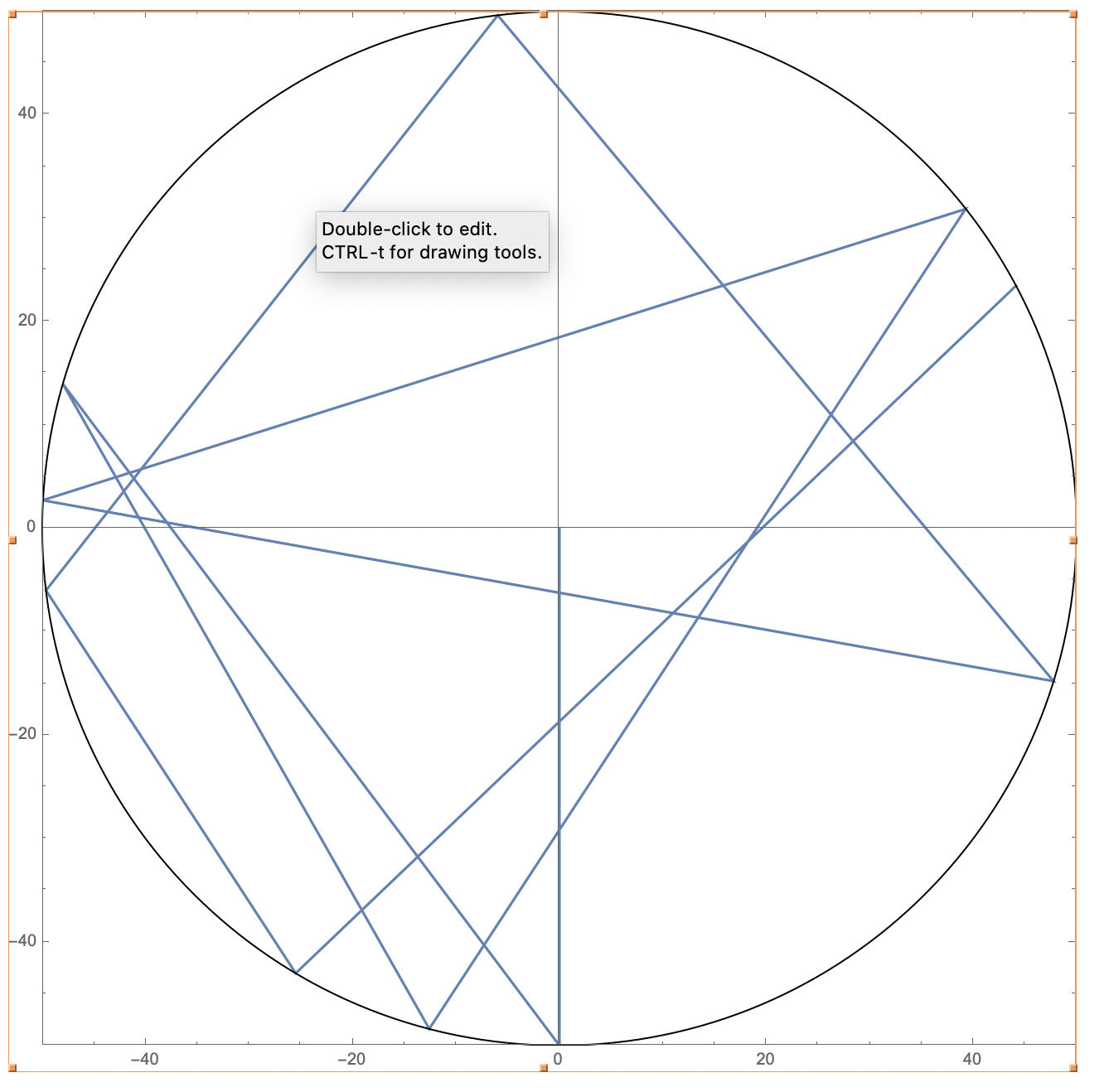
Here is a slight adaptation to my answer to your previous question here. It uses region functions, but not RegionIntersection. Rather it relies on the ray advancing to within the collision margin and using RegionNearest to approximate a reflection angle. It also counts the hits so that you could use it decay the photons as well. I have not added any scattering component and I did not join the lines. Below we will setup a simple but more complex geometry to see how it generalizes.
(* Create and Discretize Region *)
disks = RegionUnion[Disk[{-1, 0}, 0.5], Disk[{1, 0}, 0.5],
   Disk[{0, -1}, 0.5], Disk[{0, 1}, 0.5], Disk[{0, 0}, 0.25]];
region = RegionDifference[Disk[], disks];
R2 = RegionBoundary@DiscretizeRegion[region, AccuracyGoal -> 5];
(* Set up Region Operators *)
rdf = RegionDistance[R2];
rnf = RegionNearest[R2];
(* Time Increment *)
dt = 0.001;
(* Collision Margin *)
margin = 1.02 dt;
(* Starting Point for Emission *)
sp = 0.85 Normalize[{1, 1}];
(* Conditional Particle Advancer *)
advance[r_, x_, v_, c_] :=
 Block[{xnew = x + dt v}, {rdf[xnew], xnew, v, c}] /; r > margin
advance[r_, x_, v_, c_] :=
 Block[{xnew = x , vnew = v, normal = Normalize[x - rnf[x]]},
   vnew = Normalize[v - 2 v.normal normal];
   xnew += dt vnew;
   {rdf[xnew], xnew, vnew, c + 1}] /; r <= margin
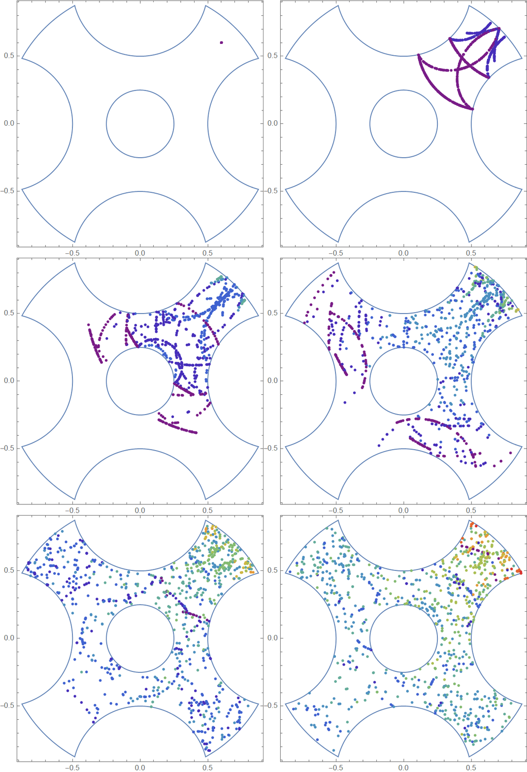
Now, setup and run the simulation and display the results.
(* Setup and run simulation *)
nparticles = 1000;
ntimesteps = 2500;
tabres = Table[
   NestList[
    advance @@ # &, {rdf[sp],
     sp, {Cos[2 Pi #], Sin[2 Pi #]} &@RandomReal[], 0},
    ntimesteps], {i, 1, nparticles}];
frames = Table[
   Rasterize@
    RegionPlot[R2,
     Epilog -> ({ColorData["Rainbow", (#4 - 1)/10],
          Disk[#2, 0.01]} & @@@ tabres[[All, i]]),
     AspectRatio -> Automatic], {i, 1, ntimesteps, 50}];
ListAnimate@frames

It took about 20s to solve the 1000 photons system on my laptop. Rendering the animation took additional time.
Extended Workflow to Include 3D Shapes
Mathematica 12.1 introduced a link to the open source 3D CAD package, OpenCascade, as described here. Being a 3D CAD modeler, OpenCascade does a pretty good job preserving sharp features efficiently. I will describe a couple of workflows to incorporate this new feature to perform 3D Raytracing with a simple solver.
Using OpenCascadeLink to Create 3D Shapes
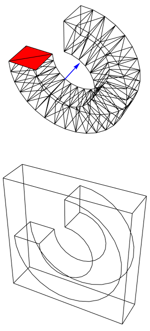
Through experimentation, I found that I needed to invert the surface normals to get the RegionDistance and RegionNearest functions to work properly. This can be done relatively simply by creating a cavity in a bounding object with the shape of interest. Here, we will create a rectangular toroidal conduit and perform the necessary differencing operation to create the cavity.
(* Load Needed Packages *)
Needs["OpenCascadeLink`"]
Needs["NDSolve`FEM`"]
(* Create a swept annular conduit *)
pp = Polygon[{{0, 0, 0}, {1, 0, 0}, {1, 1, 0}, {0, 1, 0}}];
shape = OpenCascadeShape[pp];
OpenCascadeShapeType[shape];
axis = {{2, 0, 0}, {2, 1, 0}};
sweep = OpenCascadeShapeRotationalSweep[shape, axis, -3 \[Pi]/2];
bmsweep = OpenCascadeShapeSurfaceMeshToBoundaryMesh[sweep];
(* Visualize Sweep *)
Show[Graphics3D[{{Red, pp}, {Blue, Thick, Arrow[axis]}}],
 bmsweep["Wireframe"], Boxed -> False]
(* Create Padded Bounding Box as Main Body *)
shapebb =
  OpenCascadeShape[
   Cuboid @@
    Transpose[
     CoordinateBounds[Transpose@bmsweep["Bounds"], Scaled[.05]]]];
(* Difference Padded BB from sweep in OpenCascade *)
diff = OpenCascadeShapeDifference[shapebb, sweep];
(* Visualize Differenced Model *)
bmeshdiff = OpenCascadeShapeSurfaceMeshToBoundaryMesh[diff];
bmeshdiff["Edgeframe"]
(* Create Mesh Regions *)
bmr = BoundaryMeshRegion[bmsweep];
mrd = MeshRegion[bmeshdiff];

Now, execute the simulation workflow:
(* Set up Region Operators on Differenced Geometry *)
rdf = RegionDistance[mrd];
rnf = RegionNearest[mrd];
(* Setup and run simulation *)
(* Time Increment *)
dt = 0.004;
(* Collision Margin *)
margin = 1.004 dt;
(* Conditional Particle Advancer *)
advance[r_, x_, v_, c_] :=
 Block[{xnew = x + dt v}, {rdf[xnew], xnew, v, c}] /; r > margin
advance[r_, x_, v_, c_] :=
 Block[{xnew = x , vnew = v, normal = Normalize[x - rnf[x]]},
   vnew = Normalize[v - 2 v.normal normal];
   xnew += dt vnew;
   {rdf[xnew], xnew, vnew, c + 1}] /; r <= margin
(* Starting Point for Emission *)
sp = {3, 0.5, 1};
nparticles = 2000;
ntimesteps = 2000;
tabres = Table[
   NestList[
    advance @@ # &, {rdf[sp],
     sp, { Cos[2 Pi #[[1]]] Sin[Pi #[[2]]],
        Sin[ Pi #[[2]]] Sin[2 Pi #[[1]]], Cos[ Pi #[[2]]]} &@
      First@RandomReal[1, {1, 2}], 0}, ntimesteps], {i, 1,
    nparticles}];
frames = Table[
   Rasterize@
    Graphics3D[{White, EdgeForm[Thin], Opacity[0.25], bmr,
       Opacity[1]}~
      Join~({ColorData["Rainbow", (#4 - 1)/10], Sphere[#2, 0.025]} & @@@
         tabres[[All, i]]), Boxed -> False,
     PlotRange -> RegionBounds[bmr],
     ViewPoint -> {1.5729625965895664`, -2.8428921412097794`, \
-0.9453850766634118`},
     ViewVertical -> {-0.26122960866834294`, -0.9511858016078727`,
       0.16433095379316984`}], {i, 1, ntimesteps, 66}];
ListAnimate@frames

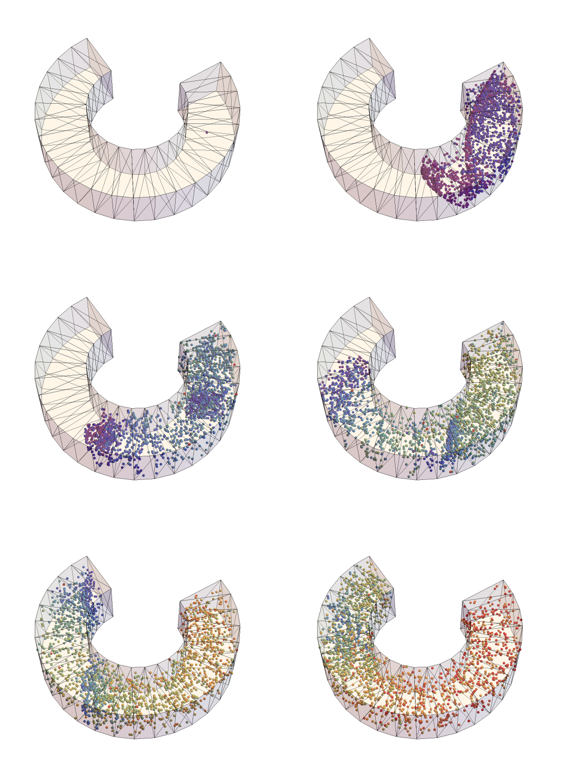
The simulation looks relatively reasonable. It will not be so fast as to be able to perform the simulations interactively, but a 2,000 particle simulation takes a minute or two. There is still plenty of room for optimization too.
Using Imported CAD
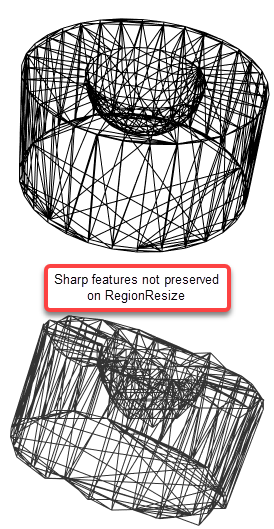
I created a hemispherical "mirror" in the SolidWorks 3D CAD package and saved the geometry as an ACIS step file. In my case, the default export was in $mm$ so I wanted to rescale back to meters. I thought RegionResize would be the approach, but it did not preserve sharpe features as shown in the following:
(* Write a ACIS step file in Current Notebook Directory *)
steptxt =
  Uncompress[
   "1:eJzVXPtv4zYS7p/iQw5wUiQGZ/juQT9obW1i1LEN29kHUMDIbXLX4PZRpGkP99/\
fUI4o0ZaoyLEX6GbXmzgUOSSH33zzoP/2z2+LZW/2ww/\
j5ewCGGf8AuEfvzDAqywdZYv827fjSbYeZcvhYjxfjWfT3ulpf7nK5r10jiD6Z+d96J+\
VLafpddY77f96/+Xhy8Pj47fHgWvcP+8jQ3bBxAWYFbM/SfYT6v75aZ86yF/\
6y//mveKAUePlt88Pd++/Pf7n9557jt6pjrEcXmXXqRMkvVnNrmer8btcxPHltH+\
2aZdNR8tsmH/\
7y09vecpH6SrNfzyBJBtdZuvJbDYnQaezaUZynBg8PwG05yfIBX1n8bmjE0zSD+\
MlrueTdJhdZ9PVmo/8cyeaGqOR9I1+bs+T0XiRDTdLVXTPBmz3z/\
lFw9tQ83YhjkiWN4u3JMp6OR7Ry+\
rjxK23mwKAbyU3cxzeLN5lpbCgSFDJSWLNz3uD1eC5tUqus+\
FVOh0P08nzOq4vs9l1tlqMh+v5IlvStFM3o/Uiq/74PLDAM+\
oT2XN3OqG1mlbGVfj8G5MM08WKBkin6/\
lsPF21rRC3A64Z00YLBlILA4Kf1zYtZm6TdxkN8WGr/\
xOUhXjAukrR4d1CDIDjTxWwYa5CFC14MhlXd0Ia0gJhil+LZLYY02Zmo7XTF9+\
u96P7e4LKkpq8LdQEZHJaqkWoCevhjLr5QELws97lZPaGNOlmOiTxUhLt4zpdOq2icXy7U\
+penlUaj1cNrRRJYoEE19S8adhnyfvvZ4uf0+WcDkjfr5NKhh9pHUaLXMGfz0+\
5KMbWLn7xtE5OHaiNchF7p70fz3rL8fMPf6f1IdhapCPa5wH9YjYZj9bp9JJQatPCC2Hia\
y10sNQ2GY4Xw0n18Ap1DnagjGTcFsIKLGAH2e4TRpwLNsjnwzgIq5hCqwrlQGhQH+\
DFUUHcPsog/IA8yWFodkPzX7+\
Z3UwrsAhVeEERhVDg2kETbbDxfcuEgH6yThdZGkAcMulxWe1OmEF0wjpJR+\
9S0srROtAA6hdlDmGB2JUdG05mS/pveZVNJtWdoz5Ndd/\
QRhYFMUBdzuosRR327wNAHGKSqFASrJOkwTrVCljf1svCk+\
X8Kms4fihies3Fd0BrLluA0AQKzdXxwZ3r5jHqlmufIUwDAFgoWtiuEyVFKCXYnEHJbFwO\
weKrD4DVMyYgOZ1k08vVVQGxvSg+\
O3uVDfxgmOSAMlqPV9l1BQKA0McRP1k05C1SYYDYIqKnYmCBVgUt/\
ZVu1xTY7AJk02pd1IJYMZAsGaCbyPpmmTrpeoM3s9XVoOckKwy8UDGMDkFA6FrOiOC4k+\
PFImxuoqDOcyadP+YXtLMydVdpyZJTogSk1kvHDt6kS68X/\
fF0eOXIqD3rRdSHLJz1vcHLufzLwdL33gV1a32CFtiVvMnAy8IkSrFLbnKLH3KY8EAVbKf\
oQ26UbFu9kFX1Raq2Q26C5uRELGajm+EqcCaJ4AU/bNwe8KJ0djAaVruWDxaDNLsYhZ+\
jWCPTEMqhDA/siYLkWSOvs5QOd7Z+P/bqGf7GTQMJQ6p/jHXIJQrQVnGPFTkjhHc+\
rndZFW/CRG1zWuTnJXY5l4YYe1ayabGgIJmqszVtgM0Yaqp6dMsdYkIpG+\
iqMq8991EXXtkDbDeiKtxtdhAHRTt3YLiaLap7K2J7q+\
OKBmQ5rKP2pjBHujY2Ug9te7A4/\
T2oopYd4jsvn5nvvg0mUVU1VeujaqrucBD2mKt9gUvsp2pq3aXDOSkGmmNmREBPwoU3GJf\
dBpET0yEouMc2mTYH26G9dESOFUfRyMK+rkfZ2zEhgeNLb2eL601cJUek5Twbjt+\
OneM7u1nkZiydfszNLhlomuB0tlr/PJ29n/qJqiSdzyfk6G1FZ27/ePr25dvTw5/\
367v73x/+/\
bVfPFGrwYeCBNMSddmwjnKfbHwhmdMDshW0oUW4sSbsYk3MobWdI4N7cBSLEeJvA6ZleZs\
/UZBFK14LffETaGuh9YCE2Kra0D+\
SJ0YvxjerVclDymHq5RDuiGoX6TTeB7G23i3LXTLXHoPdBMaaCBf3EU0GcYZo+\
DnZOYd96B/\
B7xE0Z7x2YcAoAhxVNhP1UE39n3BDrE6ESyLjpzqPLVvuYB78M2qHDaGKMl1gugZS6fGba\
Q6RG9h0qSKw1j/Thk+SBWFh9l0CMgBsCxN8NJYcZJS+GfgZb8fhyRKc97/cf/\
r19uvDp9vPff8I1m6d02ZnaFEFNh+\
Ad51vnRPQNtsOuNbdzQdwsEZa5yIS6WSdfZjTANPVsvdqK3esd73k6shACKDj+r+\
tDqZWe+xzVpOFje0xySsgq8UqwZzfxMtmR40hAeJhc3IgXpSTyxPlTDlLBXsm5bApOoWl1\
XGZo4Y4inRAKsB5wlwFGIktcK8df6N/0oM9qsbQpzMnEAQ+\
AetDCc5H2DgL3IbtTXPKHiWUC9LiDm2ysWW/vHMeuzaeGuWRwCGeO0UdzTECx64OAXB+\
gPAISOX76xwW2CMVz+\
X34Ef86IAcSzsdbrGOG18Dvps9Fyaqpq0pKCYCjBGx7CrIII8MoiVWACY0XKI+\
THbAXRai3gEx2sGpezGCQNKUD8ikajnaD+auVAazC7bJstvz/t3D70+3Xz/dr28/\
ffrj8fbT/9Z/3n7+455sRS6MH1fFs0yuNETTi/\
YsXOgWFz63XMQWyifMbuCTVDhG9YX9q1I6yer5N89ZFOqQb9UnwGCAKJRQ2lpabi45Mp1d\
gGqqZ4ueVYm1qqidNGX4HmSXM7HPkZCdrUStpxHLQYCUW+VYKF1kjnlTJdVrUts0cHOBC+\
R5p5ApSbNdZkMGejK7WeTshI6J91PznNfWGZHxM6Jq47WdCiGjiqOOS6xVbXb2cDZK1Yc6\
hEMmRyKZI55Kl+2P66Q25ulA+WpB1VJHR8w7amRVi7MnA+\
VUnXO5e6QFQdkkcF0m6Ucy6BufxxmP/CQURa7FQ7oz894rCqPjYbo8qg/\
OAoJ3mHQs7gssdGR0S4WLCksSda0GHhCCdWcOvQf31OpwTEayFxOZIyfqQJtm6Bcih34Vb\
v6W4m/gv6r4pye29ANNPW/\
I3WMXdkUVclgDB6qajeeYRU5aXFam9PcMT2rLNU9PVB6bMe4Rl8epzC6eQEMXf9Y5IHswM\
x3ywPtsqGlLBMutBdft+\
ylk2f2RXTDTFszgQeINLHspDqty27qn0vaIDts27w1DUmU75Hr3CDva+\
tzHJkvtgqAijBJZmbxZZPMNwL2bjUfLikEwPPf6ys5fexOENsfJ4e2RbfHGwEns4mxEF/\
0z8cpCOobWTdb4NIS1dbnsMtR0d/90+/D5/\
q73HGhyITok5A7CTsiaa7a4CzMGxhAZbFN5V+6iwf/+RT5/\
pb8u14a6qw2y5kiqdbd3eEANkO0U4IeeQeXagXp9BSH5j0GUkHZzNaPxwjza3ePtv556D1\
+f7h+/3j49fPt6+7nnbO/d7eMdYcNuQPGcNCMP36Ifpxb1OvjsF02+\
bzkVm2xWar24fJOvFlE/i+TaGYVaEOsz1JGkdw0dN6IuggPX5AgaTXyLDSwP/\
xCnKbqOXVy6eHlNOA4EMI2kElKq/IsbV43spxC7u3TQUmYirke1QggN+\
WTHnEkzXOQISl6PXRKBe7ispARxUAhvGZDLHrvCEWYlECK+\
f17EyWXYvi3zjDpsX4LsIpuk7jGf+\
6WfLmeLj9TFb7ePT892WnrflVTtwEkqrV6QpJIux0M7rdl+\
GSrskrrbA5IRyx3LTfTyKp1nu3a1WvB86gy6Y7u5nZW+q3o9R+HgD/\
J4ri3HFclmpIqx3B6UdAarhb+IMlZQFLgWiK+\
KYpFtORqCotlJDKAysTAWom29UQCct1wpqIBr96zdHoki5EcNjiHvXA20TwAEeaT6QwwM4\
bUQzBKJpC/a29yKNUwnluRE3nIPdpP9KRWcy9h9NvJZoxc1udq+\
VInGX7jkLTGy3ESUtJHXF0S4cprcGwAbCt6hJGIflinYEXmcUX4YeMmFscr905ZCdRcWyF\
NJohyC7yKFiSOFELHYmwhVSBw3fEAzOXL/\
EbrhbBPKIJpLlqhly6wI2++mcE30nijKCLA2stbaeECcs0qI1cZpf5JlBCMPdIGTaEBL4b\
fjCtyVsZRiRe8pHg5TpWwpHBEYPU2yVoEPVReO8jvUOaA0f9E0MTbfcdNFThDVbul7fEvr\
M3YHrGtAFTtzA2SSK2BEMA26L7XBgO3DyDWolo1tSN6hux8AotKuhVjY0DyrQ1ZZKPXS5A\
Q1bb81C3GKS7pezlrvKIaOUyIVD/nRaSVO49aWG/9IpC4+z0iADB1ezRo+\
UwIqous2ZmFDM65fHcCIWlm9/\
fkt7rNQQPojqFvyFpzWzP0DKD8D49iXLFAfmXroXfUCFs0804FvSgkhcx/\
gJJyLvFEad2ER3XtQxi90pOq+0WbW2ouoyTQsnu91okF+7cNPrOnSGm7KeVgYUDK7H+di/\
Rk0nUvt9/LpTAskhoe2Pst2SG01nW8fd88hoWnx6nDLrTNxPAR3OQfdiy/\
OwJcl3MqVtV2uU+61srYmBdw5M2CxLreTx6/K4J1HAa/\
Mlje6J6DzTyszVRex8mlx9O3Fzsfh/R/akrQ5"];
SetDirectory[NotebookDirectory[]];
file = OpenWrite["hemimirror2.step"];
WriteString[file, steptxt];
Close[file];
(* Import step file Using OpenCascade *)
shape2 = OpenCascadeShapeImport[
   "E:\\WolframCommunity\\hemimirror.step"];
bmesh2 = OpenCascadeShapeSurfaceMeshToBoundaryMesh[shape2]
bmesh2["Wireframe"]
(* Convert into MeshRegion *)
mrd = MeshRegion[bmesh2, PlotTheme -> "Lines"];
(* Scale to Meters *)
mrd = RegionPlot3D[RegionResize[mrd, 1/1000], Mesh -> All,
  PlotStyle -> None, Boxed -> False]

As you can see, RegionResize did not keep sharp feature edges on a simple uniform scaling. It is straight forward to rescale a BoundaryMesh as shown here:
(* Import step file Using OpenCascade *)
shape2 = OpenCascadeShapeImport["hemimirror2.step"];
bmesh2 = OpenCascadeShapeSurfaceMeshToBoundaryMesh[shape2]
(* Scale coordinates to meters using ToBoundaryMesh *)
bmesh2 = ToBoundaryMesh["Coordinates" -> bmesh2["Coordinates"]/1000,
  "BoundaryElements" -> bmesh2["BoundaryElements"]]
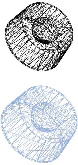
bmesh2["Wireframe"]
mrd = MeshRegion[bmesh2, PlotTheme -> "Lines"]

The simple rescaling on the BoundaryMesh preserves the sharp edges.
Now, exectute the workflow on the imported CAD.
(* Set up Region Operators on Differenced Geometry *)
rdf = RegionDistance[mrd];
rnf = RegionNearest[mrd];
(* Setup and run simulation *)
(* Time Increment *)
dt = 0.002;
(* Collision Margin *)
margin = 1.004 dt;
(* Conditional Particle Advancer *)
advance[r_, x_, v_, c_] :=
 Block[{xnew = x + dt v}, {rdf[xnew], xnew, v, c}] /; r > margin
advance[r_, x_, v_, c_] :=
 Block[{xnew = x , vnew = v, normal = Normalize[x - rnf[x]]},
   vnew = Normalize[v - 2 v.normal normal];
   xnew += dt vnew;
   {rdf[xnew], xnew, vnew, c + 1}] /; r <= margin
(* Starting Point for Emission *)
sp = {0.5, 0.25, 0};
nparticles = 2000;
ntimesteps = 4000;
tabres = Table[
   NestList[
    advance @@ # &, {rdf[sp],
     sp, { Cos[2 Pi #[[1]]] Sin[Pi #[[2]]],
        Sin[ Pi #[[2]]] Sin[2 Pi #[[1]]], Cos[ Pi #[[2]]]} &@
      First@RandomReal[1, {1, 2}], 0}, ntimesteps], {i, 1,
    nparticles}];
frames = Table[
   Rasterize@
    Graphics3D[{White, EdgeForm[Thin], Opacity[0.25], mrd,
       Opacity[1]}~
      Join~({ColorData["Rainbow", (#4 - 1)/10],
          Sphere[#2, 0.0125]} & @@@ tabres[[All, i]]), Boxed -> False,
      PlotRange -> RegionBounds[mrd],
     ViewPoint -> {0.8544727985513026`,
       2.0153230313799515`, -2.5803777467117928`},
     ViewVertical -> {-0.028824747767816083`, 0.9942988180484538`,
       0.10265960424416963`}], {i, 1, ntimesteps, 250}];
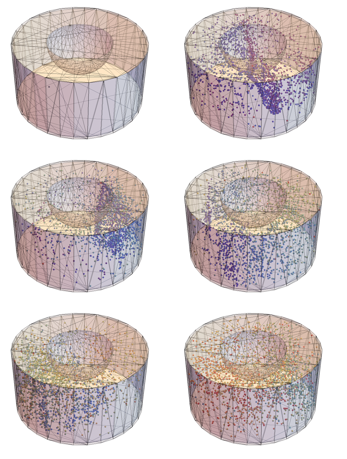
ListAnimate@frames

So, the workflow with some subtle workarounds is able to perform some sort of raytracing 3D shapes including third party CAD packages. It is only a quick and dirty prototype with room for improvement, but it's a start.

