0
$\begingroup$

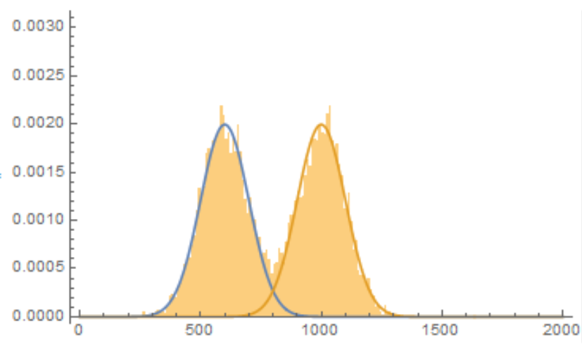
Suppose I have a dataset that is derived from a random sampling from a mixture distribution

data = RandomVariate[MixtureDistribution[{.5, .5}, {NormalDistribution[600, 100], NormalDistribution[1000, 100]}], 10000];

Show[Histogram[data, {0, 5000, 10}, "PDF", PlotRange -> {{0, 2000}, {0, .003}}], 
Plot[{.5 PDF[NormalDistribution[600, 100]][x],.5 PDF[NormalDistribution[1000, 100]][x]}, {x, 0, 2000},
PlotRange -> {{0, 2000}, {0, .003}}]]

Example Data

I'd like to partition the binned data into two separate sets respective to the two PDFs, lets say subdata1 and subdata2 so that when I run

Histogram[{subdata1,subdata2},{0,5000,10}]

I can obtain two separate normal distributions. The nature of my real data is such that it doesn't matter which distribution the overlapping region goes to, so long as those shared bins are partitioned proportionally to each PDF.

Edit 1: Changed wording from "independent" to the more correct "separate".

$\endgroup$
4
  • 1
    $\begingroup$ Would you elaborate as to why you need to assign the observations to proportionally or even assign observations at all? Typically one would have observations with known assignments and perform some classification procedure (discriminant analysis, Classify, etc.). However, you just have a sample from a mixture distribution with no known assignments. The answer I give below extracts the estimates of the parameters of the two distributions (assuming the individual distributions are Gaussian). $\endgroup$
    – JimB
    Commented Oct 30, 2018 at 23:37
  • $\begingroup$ Hi again JimB! So my real data is exactly as your answer suggests - I fit a mixture distribution to my dataset to identity two subpopulations (I actually have another issue regarding the fitting that you could probably help with, but I'm not sure it warrants a post on its own - I'll ask as a comment on your answer). I know from a control experiment that one of the populations is "poisoning" or "dirtying" my data and I want to remove this population to perform further statistics on the remaining one. In actuality, the two distributions are more closer to log-normal. $\endgroup$
    – tquarton
    Commented Oct 31, 2018 at 1:24
  • $\begingroup$ I actually found a crude solution, let me write it up for you to take a look at @JimB . $\endgroup$
    – tquarton
    Commented Oct 31, 2018 at 3:00
  • 1
    $\begingroup$ I see the purpose of the estimates of the parameters of the mixture distribution as the answer to describe the two subpopulations (what they are and what percentage each one represents). That's the answer. There's no need (in my limited imagination) to take things further by artificially assigning the data points to one of the subpopulations. The data has already done it's job by estimating the parameters. $\endgroup$
    – JimB
    Commented Oct 31, 2018 at 4:44

2 Answers 2

1
$\begingroup$

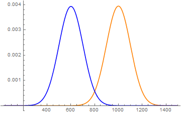
It would seem that if you do have a mixture of normal distributions, you'd want to estimate the parameters of that mixture distribution and then plot the resulting separate (rather than "independent") normal distributions:

(* Generate some data *)
SeedRandom[12345];
data = RandomVariate[MixtureDistribution[{.5, .5}, 
  {NormalDistribution[600, 100], NormalDistribution[1000, 100]}], 10000];

(* Find estimates of the parameters *)
sol = FindDistributionParameters[data, MixtureDistribution[{w1, 1 - w1},
  {NormalDistribution[μ1, σ1], NormalDistribution[μ2, σ2]}]]
(* {w1 -> 0.506919, μ1 -> 1000.2, σ1 -> 101.253, μ2 -> 601.28, σ2 -> 101.585} *)

Now plot the resulting normal distributions:

{xmin, xmax} = MinMax[data];
xlower = xmin - 0.1 (xmax - xmin);
xupper = xmax + 0.1 (xmax - xmin);
Show[
 Plot[PDF[NormalDistribution[μ1, σ1], x] /. sol,
  {x, xlower, xupper}, PlotStyle -> Orange],
 Plot[PDF[NormalDistribution[μ2, σ2], x] /. sol,
  {x, xlower, xupper}, PlotStyle -> Blue]
 ]

Two normal distributions

$\endgroup$
3
  • $\begingroup$ Please see my above comment for further detail. One issue I'm having with using `FindDistributionParameters' and 'MixtureDistribution' is that the parameters which estimate the weights of each distribution do not always sum to 1. Namely, if I have three distributions mixed, FindDistributionParameters[{a,b,c},{NormalDistribution[m1,s1],NormalDistribution[m2,s2],NormalDistribution[m3,s3]},{a,b,c,m1,s1,m2,s2,m3,s3}]. For two distributions its easy, just set a=1-b. But what about 3 distributions? How can I add the constraint a+b+c=1? $\endgroup$
    – tquarton
    Commented Oct 31, 2018 at 1:32
  • 2
    $\begingroup$ @tquarton - Then there is one additional parameter and the weights are {a, b, 1-a-b} $\endgroup$
    – Bob Hanlon
    Commented Oct 31, 2018 at 1:40
  • $\begingroup$ Ah, simple enough. I'll give it a try. $\endgroup$
    – tquarton
    Commented Oct 31, 2018 at 2:06
0
$\begingroup$

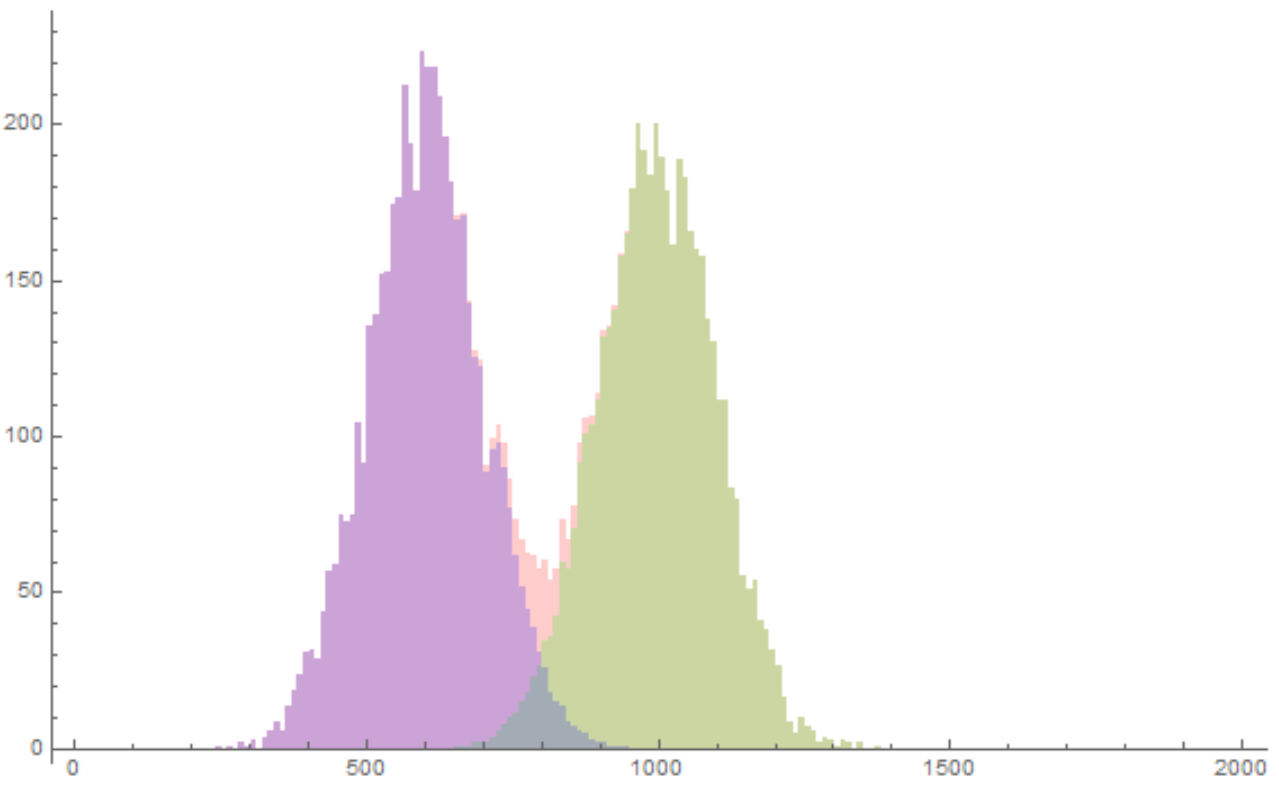
Here is my crude solution. It entails evaluating the relative weight of each PDF at a given bin and distributing the datapoints within each bin accordingly.

(* Generate some data *)
SeedRandom[12345];
data = RandomVariate[MixtureDistribution[{.5, .5}, 
{NormalDistribution[600, 100], NormalDistribution[1000, 100]}], 10000];

(* Find estimates of the parameters *)
params = FindDistributionParameters[data, MixtureDistribution[{w1, 1 - w1},
{NormalDistribution[μ1, σ1], NormalDistribution[μ2, σ2]}]]
(* {w1 -> 0.506923, μ1 -> 1000.2, σ1 -> 101.254, μ2 -> 601.278, σ2 -> 101.584} *)

First, I save the BinList and HistogramList of data for future use making suer to use the same bin criteria.

hlist=HistogramList[data,{0,5000,10}];
blist=BinLists[data,{0,5000,10}];

I then find the midpoint of the histogram bins by iterating through HistogramList bin ranges.

midpoints = 
Table[(hlist[[1, i]] + hlist[[1, i + 1]])/2, {i, 1, Length[hlist[[1]]] - 1}];

Then, I prepare to divvy up the elements of data by calculating the relative probability of the fitted PDFs evaluated at the bin midpoints.

portion1 =Table[Round[PDF[NormalDistribution[μ1, σ1]][midpoints[[i]]]/
(PDF[NormalDistribution[μ1, σ1]][midpoints[[i]]] + 
PDF[NormalDistribution[μ2, σ2]][midpoints[[i]]] + 
.000001)*hlist[[2, i]] /. params, 1], {i, 1, Length[midpoints]}];

I then take the portions of datapoints from the BinList data and save them as their own variables.

hist1 = Table[Take[blist[[i]], portion1[[i]]], {i, 1, Length[blist]}]
hist2 = Flatten[Table[Take[blist[[i]], {portion1[[i]] + 1,Length[blist[[i]]]}], {i, 1, Length[blist]}]];

and voila,

Histogram[{data, hist1, hist2}, {0, 2000, 10}, 
ChartStyle -> {Directive[Red, Opacity[.2]], Directive[Green, Opacity[.2]], Directive[Blue, Opacity[.2]]}]

histos

Edit 1: Cleaning.

$\endgroup$
4
  • 1
    $\begingroup$ This certainly accomplishes what you asked and so should be the accepted answer. But I'm not following why you'd want to do so (not that clearing up my confusions is even needed). One uses data to make inferences about some model of the world. All I'm seeing is data manipulation without a question to be answered being considered. $\endgroup$
    – JimB
    Commented Oct 31, 2018 at 4:39
  • $\begingroup$ I see your point in that having the estimated distribution is sufficient for my downstream analysis of this random variable - if I needed a discretized dataset I could just sample that very same PDF of my population of interest. However, my real data has more dimensions to it so it's important for me to select the data of interest using by separating in this dimension as a filtering or criterion. The existence and removal of the population being removed is validated using a secondary control experiment. The nature of the instrument collecting the data inserts junk datapoints in my dataset. $\endgroup$
    – tquarton
    Commented Oct 31, 2018 at 14:11
  • 1
    $\begingroup$ So it sounds like you might want to consider an initial cluster analysis for your multidimensional data (unless you already know how many clusters should exist). $\endgroup$
    – JimB
    Commented Oct 31, 2018 at 14:33
  • $\begingroup$ Having thought more about it, I suppose a multidimensional clustering is probably more appropriate being that clustering will also take into account the higher dimensions. By limiting myself to just this dimension I'd be losing some potentially useful information used to define my population of interest. Thanks as always JimB. $\endgroup$
    – tquarton
    Commented Oct 31, 2018 at 14:48

Your Answer

By clicking “Post Your Answer”, you agree to our terms of service and acknowledge you have read our privacy policy.

Not the answer you're looking for? Browse other questions tagged or ask your own question.