Consider a linear system .
bandPassOL[omega_, k_] := Module[{a, b, c, d},
  a = {{0, -omega}, {omega, 0}};
  b = {{omega*k}, {0}};
  c = {{1, 0}, {0, 1}};
  d = {{0}, {0}};
  StateSpaceModel[{a, b, c, d}]
](*Module*)
osg2SSOL = SystemsModelParallelConnect[bandPassOL[omega1, k1],
   bandPassOL[omega2, k2], All, None];
osg2SSCL = SystemsModelFeedbackConnect[osg2SSOL, {{1, 1}, {3, 1}}];
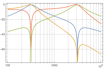
If I want to plot frequency characteristic of such a SIMO system using BodePlot
BodePlot[osg2SSCL /. {k1 -> 0.5,
   k2 -> 0.5, omega1 -> 2 Pi 50, omega2 -> 2 Pi 500}, {10^2, 10^4}, GridLines -> Automatic,
   PlotLayout -> "Magnitude"]
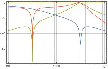
I get the following, incorrect result.
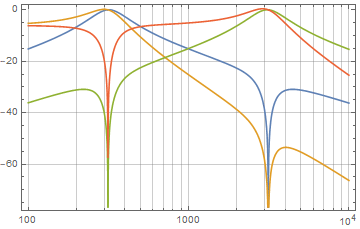
If, on the other hand, I wrap the system with TransferFunctionModel and send it to BodePlot
BodePlot[TransferFunctionModel[osg2SSCL, s] /. {k1 -> 0.5,
   k2 -> 0.5, omega1 -> 2 Pi 50, omega2 -> 2 Pi 500}, {10^2, 10^4}, GridLines -> Automatic,
   PlotLayout -> "Magnitude"]
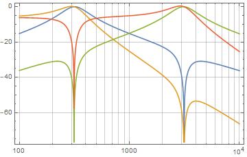
I get the correct result.
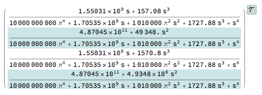
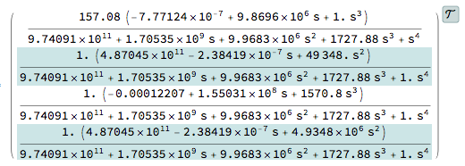
If I vary coefficients k1 and k2 from 0.01 to 1, the difference between outputs varies. For small values of k1 and k2, the difference is large and easy to spot, but as k1 and k2 approach 1 the difference gets smaller and easy to miss.
I've tried several other systems and seems that the errors starts to appear only if the system has more than 3 outputs. Though this was far from extensive verification.
Should this be considered a bug?
The problem persist through the following versions of MMA
"11.2.0 for Microsoft Windows (64-bit) (September 11, 2017)"
"10.2.0 for Microsoft Windows (64-bit) (July 28, 2015)"
"11.3.0 for Microsoft Windows (64-bit) (March 7, 2018)"

