4
$\begingroup$

I am currently trying to plot an implicit function of the form $f(x,y) = 0$ in mathematica.

The example I am using is $f(x,y) = y^4 - 730 y^2 + x^4 + 3y^2 x^2 - 675 x^2 + 729$

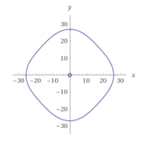
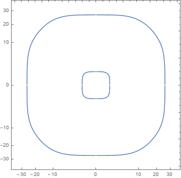
However the function has a small circle type shape at the origin and a another large circular shape around the origin:

enter image description here

This was plotted using the mathematica command:

ContourPlot[729 + x^4 + y^4 + 3 x^2 (-225 + y^2) == 730 y^2,
 {x, -32, 32}, {y, -34, 34}]

Question: is there some way to make the plot so that the smaller circle becomes more visible?

$\endgroup$
1
  • $\begingroup$ This seems related: (18866) $\endgroup$
    – Mr.Wizard
    Commented Jul 29, 2017 at 11:37

3 Answers 3

4
$\begingroup$

Revising this answer I propose extracting contours from ContourPlot, converting to polar, scaling magnitude, then converting back and plotting. I will use code from ListLogLinearPlot for the whole real numbers:

logify[_][x_ /; x == 0] := 0
logify[off_][x_] := Sign[x] Max[0, (off + Re@Log@x)/off]

inverse[off_][x_] := Sign[x] Exp[(Abs[x] - 1) off]

logscale[n_] := {logify[n], inverse[n]}

And an auxiliary function:

logTheta[m_][pts_] :=
  FromPolarCoordinates /@ 
    MapAt[logify[m], ToPolarCoordinates /@ pts, {All, 1}];

Now:

cp = ContourPlot[
   729 + x^4 + y^4 + 3 x^2 (-225 + y^2) == 730 y^2, {x, -32, 32}, {y, -34, 34}, 
   MaxRecursion -> 3];

pts = Cases[Normal @ cp, Line[x_] :> x, -3];

ListLinePlot[logTheta[2] /@ pts
  , Ticks -> Charting`ScaledTicks @ logscale[2]
  , AspectRatio -> 1
]
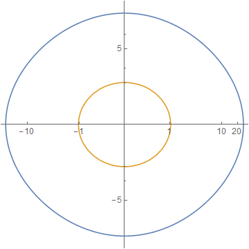
enter image description here

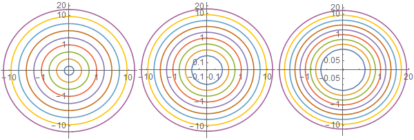
An additional example to better illustrate variable "zoom" in the scaling:

cp2 = ContourPlot[
  Evaluate[x^2 + y^2 == # & /@ (3^Range[-3, 5])], {x, -16, 16}, {y, -16, 16}, 
  PlotPoints -> 50]

pts2 = Cases[Normal@cp2, Line[x_] :> x, -3];

ListLinePlot[logTheta[#] /@ pts2
 , Ticks -> Charting`ScaledTicks @ logscale[#]
 , AspectRatio -> 1
] & /@ {2, 3, 4}
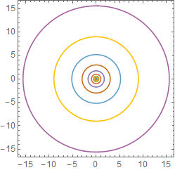
enter image description here

enter image description here

Beware: if the "zoom" is not enough you'll create singularities in the polar/Cartesian conversion and get errors instead of a plot:

logTheta[1] /@ pts2;

FromPolarCoordinates::bdpt: Evaluation point {0,1.92728} is not a valid set of polar or hyperspherical coordinates. >>

I expect this will be a problem if you have contours that cross the origin, but I will have to come back to that later.

Controlling tick marks

Here is a way to "manually" generate a specification for Ticks or FrameTicks.

cp = ContourPlot[
   729 + x^4 + y^4 + 3 x^2 (-225 + y^2) == 730 y^2, {x, -32, 32}, {y, -34, 34}, 
   MaxRecursion -> 3];

pts = Cases[Normal@cp, Line[x_] :> x, -3];

log = logTheta[2] /@ pts;

ticks = {#, inverse[2][#]} & /@ FindDivisions[#, 11] & /@ CoordinateBounds[log];

ListLinePlot[log, Ticks -> ticks, AspectRatio -> 1]
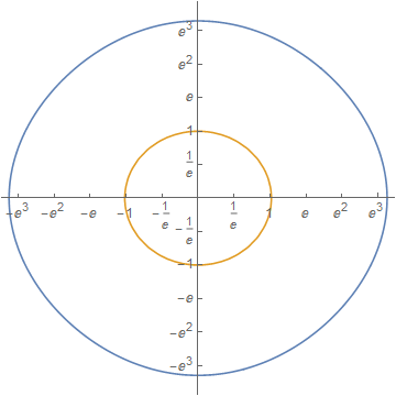
enter image description here

And for the additional example:

cp2 = ContourPlot[
  Evaluate[x^2 + y^2 == # & /@ (3^Range[-3, 5])], {x, -16, 16}, {y, -16, 16}, 
  PlotPoints -> 50]

pts2 = Cases[Normal@cp2, Line[x_] :> x, -3];

Table[
  log = logTheta[b] /@ pts2;
  ticks = {#, inverse[b][#]} & /@ FindDivisions[#, 11] & /@ CoordinateBounds[log];
  ListLinePlot[log, Ticks -> ticks, AspectRatio -> 1, ImageSize -> 200],
  {b, {2, 3, 4}}
] // Row
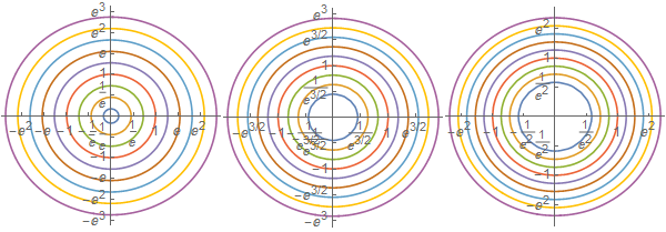
enter image description here

$\endgroup$
7
  • $\begingroup$ How would you add ticks back to these images? $\endgroup$
    – Gr Eg
    Commented Jul 30, 2017 at 10:45
  • $\begingroup$ For some reason when I copy this code, the ticks are not showing up on the image, do you perhaps know why this is? $\endgroup$
    – Gr Eg
    Commented Jul 30, 2017 at 11:25
  • $\begingroup$ @GrEg You're using the code with Ticks -> Charting`ScaledTicks @ logscale[2] right? I guess it's a version issue; which version of Mathematica are you using? I'll add code for "manual" tick generation later if I have time. $\endgroup$
    – Mr.Wizard
    Commented Jul 30, 2017 at 13:51
  • $\begingroup$ I am using the online version of mathematica from wolfram alpha. Yeah I am using that code. Thanks I would appreciate it! $\endgroup$
    – Gr Eg
    Commented Jul 30, 2017 at 14:31
  • $\begingroup$ I think the version is 11.1.1 $\endgroup$
    – Gr Eg
    Commented Jul 30, 2017 at 14:57
2
$\begingroup$

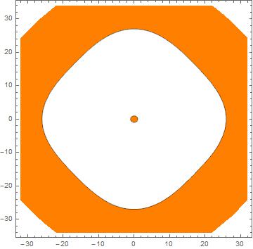
Maybe

ContourPlot[
 729 + x^4 + y^4 + 3 x^2 (-225 + y^2) - 730 y^2,
 {x, -32, 32}, {y, -34, 34},
 Contours -> {{0}},
 ContourShading -> {White, Orange}]

enter image description here

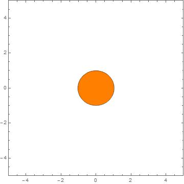
You can magnify the center circle by decreasing the PlotRange

r = 5;

ContourPlot[
 729 + x^4 + y^4 + 3 x^2 (-225 + y^2) - 730 y^2,
 {x, -32, 32}, {y, -34, 34},
 Contours -> {{0}},
 ContourShading -> {White, Orange},
 PlotPoints -> 50,
 PlotRange -> {{-r, r}, {-r, r}}]

enter image description here

$\endgroup$
3
  • 2
    $\begingroup$ Thanks for the reply, I was thinking something more along the lines of changing the scales to a logarithmic scale, but I am not sure how to do this. $\endgroup$
    – Gr Eg
    Commented Jul 29, 2017 at 11:26
  • $\begingroup$ Is there no way of setting an 'axis scale'? $\endgroup$
    – Gr Eg
    Commented Jul 29, 2017 at 11:33
  • $\begingroup$ Not with ContourPlot or RegionPlot $\endgroup$
    – eldo
    Commented Jul 29, 2017 at 11:38
1
$\begingroup$

You could rescale your variables with something like:

lhs[x_, y_] := 729 + x^4 + y^4 + 3 x^2 (-225 + y^2)
rhs[y_] := 730 y^2
ticks = {#, #} &@{Table[{Sign[i] Sqrt[Abs[i]], i}, {i, -30, 30, 10}], Automatic};

Then

ContourPlot[lhs[Sign[x] x^2, Sign[y] y^2] == rhs[Sign[y] y^2], 
  {x, -6, 6}, {y, -6, 6}, FrameTicks -> ticks]

gives

enter image description here

$\endgroup$

Your Answer

By clicking “Post Your Answer”, you agree to our terms of service and acknowledge you have read our privacy policy.

Not the answer you're looking for? Browse other questions tagged or ask your own question.