added 1270 characters in body
Source Link
Mr.Wizard
  • 273.1k
  • 34
  • 595
  • 1.4k

Controlling tick marks

Here is a way to "manually" generate a specification for Ticks or FrameTicks.

cp = ContourPlot[
   729 + x^4 + y^4 + 3 x^2 (-225 + y^2) == 730 y^2, {x, -32, 32}, {y, -34, 34}, 
   MaxRecursion -> 3];

pts = Cases[Normal@cp, Line[x_] :> x, -3];

log = logTheta[2] /@ pts;

ticks = {#, inverse[2][#]} & /@ FindDivisions[#, 11] & /@ CoordinateBounds[log];

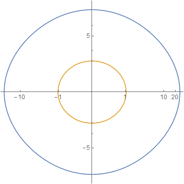
ListLinePlot[log, Ticks -> ticks, AspectRatio -> 1]

enter image description here

And for the additional example:

cp2 = ContourPlot[
  Evaluate[x^2 + y^2 == # & /@ (3^Range[-3, 5])], {x, -16, 16}, {y, -16, 16}, 
  PlotPoints -> 50]

pts2 = Cases[Normal@cp2, Line[x_] :> x, -3];

Table[
  log = logTheta[b] /@ pts2;
  ticks = {#, inverse[b][#]} & /@ FindDivisions[#, 11] & /@ CoordinateBounds[log];
  ListLinePlot[log, Ticks -> ticks, AspectRatio -> 1, ImageSize -> 200],
  {b, {2, 3, 4}}
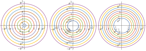
] // Row

enter image description here

deleted 363 characters in body
Source Link
Mr.Wizard
  • 273.1k
  • 34
  • 595
  • 1.4k

At least in v10.1 ContourPlot doesn't supportRevising this answer I propose extracting contours from ScalingFunctionsContourPlot, but ListLinePlot doesconverting to polar, unofficiallyscaling magnitude, then converting back and plotting. Therefore this might be of some I will use.

Using logscale code from ListLogLinearPlot for the whole real numbers  :

logify[_][x_ /; x == 0] := 0
logify[off_][x_] := Sign[x] Max[0, (off + Re@Log@x)/off]

inverse[off_][x_] := Sign[x] Exp[(Abs[x] - 1) off]

logscale[n_] := {logify[n], inverse[n]}

And an auxiliary function:

logTheta[m_][pts_] :=
(* additional definitionFromPolarCoordinates *)/@ 
logscale[n_, m_] := logscale MapAt[logify[m], ToPolarCoordinates /@ pts, {nAll, m1}];
cp = ContourPlot[
   729 + x^4 + y^4 + 3 x^2 (-225 + y^2) == 730 y^2, {x, -32, 32}, {y, -34, 34}, 
   MaxRecursion -> 3];

pts = Cases[Normal@cpCases[Normal @ cp, Line[x_] :> x, -3];

ListLinePlot[pts,ListLinePlot[logTheta[2] ScalingFunctions/@ ->pts
 logscale[2, 2], AspectRatioTicks -> 1]
enter image description here

You can change the numeric parameters in logscale to get different effects; see the linked post for further examples.

Working in polar coordinates makes things look nicer, but I lose automatic tick generation so I have to turn them off:

newpts = FromPolarCoordinatesCharting`ScaledTicks /@ logscale[2]
  MapAt[logify[2], ToPolarCoordinates /@ pts, {All, All, 1}];

ListLinePlot[newpts, Ticks -> None, AspectRatio -> 1]1
]

enter image description hereenter image description here

The ticks could be calculated with inverse[2] but I don't have timeAn additional example to complete that now.

Additional examples of each methodbetter illustrate variable "zoom" in the scaling:

cp2 = ContourPlot[
  Evaluate[x^2 + y^2 == # & /@ (3^Range[-3, 5])], {x, -16, 16}, {y, -16, 16}, 
  PlotPoints -> 50]

pts2 = Cases[Normal@cp2, Line[x_] :> x, -3];

ListLinePlot[pts2, ScalingFunctionsListLinePlot[logTheta[#] ->/@ logscale[3,pts2
 3], AspectRatioTicks -> 1]
enter image description here

newpts2 = FromPolarCoordinatesCharting`ScaledTicks /@ logscale[#]
 , AspectRatio MapAt[logify[3],-> ToPolarCoordinates1
] & /@ pts2, {All2, All3, 14}];

ListLinePlot[newpts2, Ticks -> None, AspectRatio
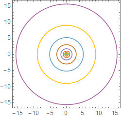
enter image description here

enter image description here

Beware: if the "zoom" is not enough you'll create singularities in the polar/Cartesian conversion and get errors instead of a plot:

logTheta[1] ->/@ Automatic]pts2;

FromPolarCoordinates::bdpt: Evaluation point {0,1.92728} is not a valid set of polar or hyperspherical coordinates. >>

enter image description here I expect this will be a problem if you have contours that cross the origin, but I will have to come back to that later.


At least in v10.1 ContourPlot doesn't support ScalingFunctions, but ListLinePlot does, unofficially. Therefore this might be of some use.

Using logscale from ListLogLinearPlot for the whole real numbers  :

logify[_][x_ /; x == 0] := 0
logify[off_][x_] := Sign[x] Max[0, (off + Re@Log@x)/off]

inverse[off_][x_] := Sign[x] Exp[(Abs[x] - 1) off]

logscale[n_] := {logify[n], inverse[n]}

(* additional definition *)
logscale[n_, m_] := logscale /@ {n, m}
cp = ContourPlot[
   729 + x^4 + y^4 + 3 x^2 (-225 + y^2) == 730 y^2, {x, -32, 32}, {y, -34, 34}, 
   MaxRecursion -> 3];

pts = Cases[Normal@cp, Line[x_] :> x, -3];

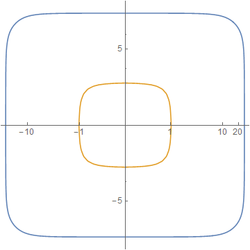
ListLinePlot[pts, ScalingFunctions -> logscale[2, 2], AspectRatio -> 1]

enter image description here

You can change the numeric parameters in logscale to get different effects; see the linked post for further examples.

Working in polar coordinates makes things look nicer, but I lose automatic tick generation so I have to turn them off:

newpts = FromPolarCoordinates /@ 
  MapAt[logify[2], ToPolarCoordinates /@ pts, {All, All, 1}];

ListLinePlot[newpts, Ticks -> None, AspectRatio -> 1]

enter image description here

The ticks could be calculated with inverse[2] but I don't have time to complete that now.

Additional examples of each method:

cp2 = ContourPlot[
  Evaluate[x^2 + y^2 == # & /@ (3^Range[-3, 5])], {x, -16, 16}, {y, -16, 16}, 
  PlotPoints -> 50]

pts2 = Cases[Normal@cp2, Line[x_] :> x, -3];

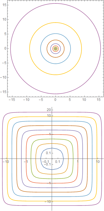
ListLinePlot[pts2, ScalingFunctions -> logscale[3, 3], AspectRatio -> 1]

enter image description here

newpts2 = FromPolarCoordinates /@ 
   MapAt[logify[3], ToPolarCoordinates /@ pts2, {All, All, 1}];

ListLinePlot[newpts2, Ticks -> None, AspectRatio -> Automatic]
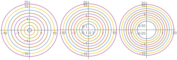
enter image description here


Revising this answer I propose extracting contours from ContourPlot, converting to polar, scaling magnitude, then converting back and plotting. I will use code from ListLogLinearPlot for the whole real numbers:

logify[_][x_ /; x == 0] := 0
logify[off_][x_] := Sign[x] Max[0, (off + Re@Log@x)/off]

inverse[off_][x_] := Sign[x] Exp[(Abs[x] - 1) off]

logscale[n_] := {logify[n], inverse[n]}

And an auxiliary function:

logTheta[m_][pts_] :=
  FromPolarCoordinates /@ 
    MapAt[logify[m], ToPolarCoordinates /@ pts, {All, 1}];
cp = ContourPlot[
   729 + x^4 + y^4 + 3 x^2 (-225 + y^2) == 730 y^2, {x, -32, 32}, {y, -34, 34}, 
   MaxRecursion -> 3];

pts = Cases[Normal @ cp, Line[x_] :> x, -3];

ListLinePlot[logTheta[2] /@ pts
  , Ticks -> Charting`ScaledTicks @ logscale[2]
  , AspectRatio -> 1
]

enter image description here

An additional example to better illustrate variable "zoom" in the scaling:

cp2 = ContourPlot[
  Evaluate[x^2 + y^2 == # & /@ (3^Range[-3, 5])], {x, -16, 16}, {y, -16, 16}, 
  PlotPoints -> 50]

pts2 = Cases[Normal@cp2, Line[x_] :> x, -3];

ListLinePlot[logTheta[#] /@ pts2
 , Ticks -> Charting`ScaledTicks @ logscale[#]
 , AspectRatio -> 1
] & /@ {2, 3, 4}

enter image description here

enter image description here

Beware: if the "zoom" is not enough you'll create singularities in the polar/Cartesian conversion and get errors instead of a plot:

logTheta[1] /@ pts2;

FromPolarCoordinates::bdpt: Evaluation point {0,1.92728} is not a valid set of polar or hyperspherical coordinates. >>
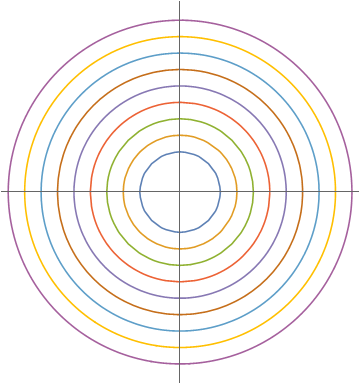
I expect this will be a problem if you have contours that cross the origin, but I will have to come back to that later.

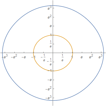
added 754 characters in body
Source Link
Mr.Wizard
  • 273.1k
  • 34
  • 595
  • 1.4k

At least in v10.1 ContourPlot doesn't support ScalingFunctions, but ListLinePlot does, unofficially. Therefore this might be of some use.

Using logscale from ListLogLinearPlot for the whole real numbers :

logify[_][x_ /; x == 0] := 0
logify[off_][x_] := Sign[x] Max[0, (off + Re@Log@x)/off]

inverse[off_][x_] := Sign[x] Exp[(Abs[x] - 1) off]

logscale[n_] := {logify[n], inverse[n]}

(* additional definition *)
logscale[n_, m_] := logscale /@ {n, m}

Now:

cp = ContourPlot[
   729 + x^4 + y^4 + 3 x^2 (-225 + y^2) == 730 y^2, {x, -32, 32}, {y, -34, 34}, 
   MaxRecursion -> 3];

pts = Cases[Normal@cp, Line[x_] :> x, -3];

ListLinePlot[pts, ScalingFunctions -> logscale[2, 2], AspectRatio -> 1]

enter image description here

You can change the numeric parameters in logscale to get different effects; see the linked post for further examples.

An additional exampleWorking in polar coordinates makes things look nicer, but I lose automatic tick generation so I have to turn them off:

newpts = FromPolarCoordinates /@ 
  MapAt[logify[2], ToPolarCoordinates /@ pts, {All, All, 1}];

ListLinePlot[newpts, Ticks -> None, AspectRatio -> 1]

enter image description here

The ticks could be calculated with inverse[2] but I don't have time to complete that now.

Additional examples of each method:

cp2 = ContourPlot[
  Evaluate[x^2 + y^2 == # & /@ (3^Range[-3, 5])], {x, -16, 16}, {y, -16, 16}, 
  PlotPoints -> 50]

pts2 = Cases[Normal@cp2, Line[x_] :> x, -3];

ListLinePlot[pts2, ScalingFunctions -> logscale[3, 3], AspectRatio -> 1]

enter image description here

newpts2 = FromPolarCoordinates /@ 
   MapAt[logify[3], ToPolarCoordinates /@ pts2, {All, All, 1}];

ListLinePlot[newpts2, Ticks -> None, AspectRatio -> Automatic]

enter image description here


At least in v10.1 ContourPlot doesn't support ScalingFunctions, but ListLinePlot does, unofficially. Therefore this might be of some use.

Using logscale from ListLogLinearPlot for the whole real numbers :

logify[_][x_ /; x == 0] := 0
logify[off_][x_] := Sign[x] Max[0, (off + Re@Log@x)/off]

inverse[off_][x_] := Sign[x] Exp[(Abs[x] - 1) off]

logscale[n_] := {logify[n], inverse[n]}

(* additional definition *)
logscale[n_, m_] := logscale /@ {n, m}

Now:

cp = ContourPlot[
   729 + x^4 + y^4 + 3 x^2 (-225 + y^2) == 730 y^2, {x, -32, 32}, {y, -34, 34}, 
   MaxRecursion -> 3];

pts = Cases[Normal@cp, Line[x_] :> x, -3];

ListLinePlot[pts, ScalingFunctions -> logscale[2, 2], AspectRatio -> 1]

enter image description here

You can change the numeric parameters in logscale to get different effects; see the linked post for further examples.

An additional example:

cp2 = ContourPlot[
  Evaluate[x^2 + y^2 == # & /@ (3^Range[-3, 5])], {x, -16, 16}, {y, -16, 16}, 
  PlotPoints -> 50]

pts2 = Cases[Normal@cp2, Line[x_] :> x, -3];

ListLinePlot[pts2, ScalingFunctions -> logscale[3, 3], AspectRatio -> 1]

enter image description here

At least in v10.1 ContourPlot doesn't support ScalingFunctions, but ListLinePlot does, unofficially. Therefore this might be of some use.

Using logscale from ListLogLinearPlot for the whole real numbers :

logify[_][x_ /; x == 0] := 0
logify[off_][x_] := Sign[x] Max[0, (off + Re@Log@x)/off]

inverse[off_][x_] := Sign[x] Exp[(Abs[x] - 1) off]

logscale[n_] := {logify[n], inverse[n]}

(* additional definition *)
logscale[n_, m_] := logscale /@ {n, m}

Now:

cp = ContourPlot[
   729 + x^4 + y^4 + 3 x^2 (-225 + y^2) == 730 y^2, {x, -32, 32}, {y, -34, 34}, 
   MaxRecursion -> 3];

pts = Cases[Normal@cp, Line[x_] :> x, -3];

ListLinePlot[pts, ScalingFunctions -> logscale[2, 2], AspectRatio -> 1]

enter image description here

You can change the numeric parameters in logscale to get different effects; see the linked post for further examples.

Working in polar coordinates makes things look nicer, but I lose automatic tick generation so I have to turn them off:

newpts = FromPolarCoordinates /@ 
  MapAt[logify[2], ToPolarCoordinates /@ pts, {All, All, 1}];

ListLinePlot[newpts, Ticks -> None, AspectRatio -> 1]

enter image description here

The ticks could be calculated with inverse[2] but I don't have time to complete that now.

Additional examples of each method:

cp2 = ContourPlot[
  Evaluate[x^2 + y^2 == # & /@ (3^Range[-3, 5])], {x, -16, 16}, {y, -16, 16}, 
  PlotPoints -> 50]

pts2 = Cases[Normal@cp2, Line[x_] :> x, -3];

ListLinePlot[pts2, ScalingFunctions -> logscale[3, 3], AspectRatio -> 1]

enter image description here

newpts2 = FromPolarCoordinates /@ 
   MapAt[logify[3], ToPolarCoordinates /@ pts2, {All, All, 1}];

ListLinePlot[newpts2, Ticks -> None, AspectRatio -> Automatic]

enter image description here

 
added 388 characters in body
Source Link
Mr.Wizard
  • 273.1k
  • 34
  • 595
  • 1.4k
Loading
Source Link
Mr.Wizard
  • 273.1k
  • 34
  • 595
  • 1.4k
Loading